Summary Statistics

You’ve got spikes… Now what? Unit I was all about extracting signals of interest from neural and behavioral measurements. Unit II is about modeling those signals to discover principles of neural computation.

A first step toward this lofty goal is to understand what makes neurons spike. Encoding models predict when neurons will fire in response to sensory stimuli or behavioral covariates. An accurate encoding model can shed light on which features of sensory inputs a neuron is most responsive or “tuned” to. A good model can reveal how tuning properties vary across a population of neurons, or how those properties change from one population to the next.

Before diving into models, though, we’ll start by discussing simple summary statistics of neural spike trains. We are often interested in the relationship between sensory inputs and neural activity. Spike triggered averages (STAs) and peri-stimulus time histograms (PSTHs) are useful summaries of these relationships. Likewise, when we are interested in the relationships between neural responses, cross-correlation functions offer simple summaries of multi-neuronal measurements. These statistics offer not only a high-level summary of neural activity, they also offer a means for checking the encoding models we’ll build later. A good model should recapitulate these basic statistics of the data.

Peri-stimulus time histogram

We will start with a discrete time formulation with equally spaced time bins of width \(\Delta\). Let,

• \(\mathbf{x}_t\) denote a stimulus (e.g. a sensory input) at time bin \(t\)

• \(\mathbf{y}_t = (y_{t,1}, \ldots, y_{t,N})\) with each \(y_{t,n} \in \mathbb{N}_0\) denote the number of spikes fired in time bin \(t\).

Note

We typically take \(\Delta\) to be relatively small, on the order of 5 ms to 100 ms. With \(\Delta = 5\) ms, you would not expect to see more than one spike per time bin. For larger bin sizes, you could see multiple spikes.

A peri-stimulus time histogram (PSTH) is a simple summary statistic of the relationship between \(\mathbf{x}\) and \(\mathbf{y}\). For simplicity, suppose the stimulus is binary so that \(x_t \in \{0,1\}\). The PSTH is an estimate of the conditional mean of \(\mathbf{y}\) at an offset from when \(x = 1\),

\[ \begin{aligned} \boldsymbol{\rho}_d &= \frac{\sum_{t=1}^T \mathbf{y}_{t+d} \, \mathbb{I}[x_t = 1]}{\sum_{t=1}^T \mathbb{I}[x_t = 1]} \approx \mathbb{E}[\mathbf{y}_{t+d} \mid x_t = 1]. \end{aligned} \]

for \(d\in \{-D, \ldots, D\}\).

Of course, typical stimuli are not binary. However, we can always define an event \(\mathcal{A}\) (in the probabilistic sense of a subset of the stimulus space) and define the PSTH as \(\boldsymbol{\rho}_d \approx \mathbb{E}[\mathbf{y}_{t+d} \mid \mathbf{x}_t \in \mathcal{A}]\).

Spike-Triggered Average (STA)

The spike-triggered average (STA) is simply the conditional expectation in the other direction,

\[ \begin{aligned} \mathbf{s}_{n,d} &= \frac{\sum_{t=1}^T \mathbf{x}_{t+d} \, \mathbb{I}[y_{t,n} = 1]}{\sum_{t=1}^T \mathbb{I}[y_{t,n} = 1]} \approx \mathbb{E}[\mathbf{x}_{t+d} \mid y_{t,n} = 1]. \end{aligned} \]

It tells you what, on average, the stimulus looks like when neuron \(n\) spikes.

Fano factor

The PSTH and STA are first moments — conditional means. Spike counts are variable though. The same stimulus might elicit different numbers of spikes on different trials. Second moments tell you the variance of those responses.

The Fano factor is a summary statistic that measures the dispersion of spike counts,

\[ F_n = \frac{\mathbb{V}[y_{t,n}]}{\mathbb{E}[y_{t,n}]} \]

If \(F_n < 1\), the counts are under-dispersed, and if \(F_n > 1\) the counts are over-dispersed. When the spike counts follow a Poisson distribution, they have unit dispersion and \(F_n = 1\).

Note that the distribution of spike counts will typically vary with the stimulus, so the Fano factor (and dispersion) should really be calculated conditionally on \(\mathbf{x}_t\). Goris et al. [2014] modeled the stimulus-dependent Fano factor with a generalized linear model (see below), and found that spike counts were increasingly overdispersed as they progressed through the hierarchy of visual brain areas. Charles et al. [2018] further generalized their approach is an attempt to “dethrone” the Fano factor.

Other measures of dispersion

The Fano factor is only one measure of the dispersion of a random variable. Another is the coefficient of variation,

\[ \mathrm{CV}_n = \frac{\sqrt{\mathbb{V}[y_{t,n}]}}{\mathbb{E}[y_{t,n}]}, \]

which is the ratio of the standard deviation to the mean. It turns out that in renewal processes, there is a relationship between the Fano factor of the spike counts and the coefficient of variation of the inter-spike intervals.

Cross-correlation function

Another second-order statistic of interest is the cross-correlation function (CCF) between a pair of neurons \((i, j)\) for varying delays \(d\),

\[ \mathbb{E}\left[ \left(\frac{y_{t,i} - \mu_i}{\sigma_i} \right) \left(\frac{y_{t+d,j} - \mu_j}{\sigma_j} \right) \right], \]

where \(\mu_i = \mathbb{E}[y_{t,i}]\) is the mean and \(\sigma_i = \sqrt{\mathbb{V}[y_{t,i}]}\) is the standard deviation of spike counts on neuron \(i\).

The cross-correlation function tells us how often neuron \(j\) spikes \(d\) time-steps before or after neuron \(i\). We often visualize the CCF is a matrix of subplots,

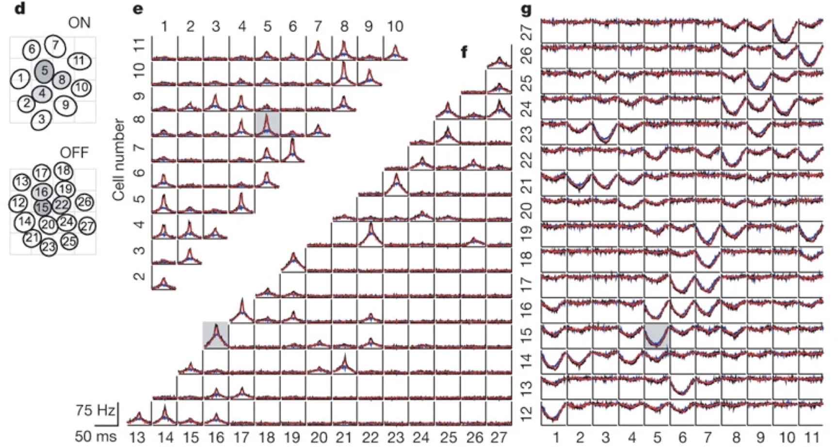
Fig. 10 A matrix of subplots showing the cross-correlation function for pairs of retinal ganglion cells. This figure is adapted from Pillow et al. [2008].

Exercise

How does the cross-correlation function defined above relate to the cross correlation operation (aka convolution in deep learning) used in Unit I?

Conclusion

Summary statistics like PSTHs, STAs, Fano factors, and CCFs offer a high-level summary of neural spike trains. They can already shed insight into how neural populations encode information about external stimuli. Next, we will talk about simple models for predicting neural spike trains.