Lab 7: Switching LDS#
STATS320: Machine Learning Methods for Neural Data Analysis
Stanford University. Winter, 2023.
Team Name: Your team name here
Team Members: Names of everyone on your team here
Due: 11:59pm Thursday, March 9, 2023 via GradeScope

In this lab, we will implement a variational expectation maximization algorithm to fit a latent variable model with both discrete and continuous states. We’ll use a mean field approximation, which we’ll fit using coordinate ascent variational inference (CAVI). Then we’ll test it out on neural activity traces extracted from calcium imaging of the worm C. elegans by Kato et al (2015), in their paper on low dimensional dynamics of whole brain activity.
We won’t implement variational EM for full-blown hierachical, recurrent, switching linear dynamical systems (Linderman et al, 2019). Instead, we’ll work on a simpler model without time dependencies, which reduces to a mixture of factor analysis models. Once we’ve done so, you’ll understand how the main fitting algorithms underlying SSM work under the hood!
References
Kato, Saul, Harris S. Kaplan, Tina Schrödel, Susanne Skora, Theodore H. Lindsay, Eviatar Yemini, Shawn Lockery, and Manuel Zimmer. 2015. “Global Brain Dynamics Embed the Motor Command Sequence of Caenorhabditis Elegans.” Cell 163 (3): 656–69.
Linderman, Scott W., Annika L. A. Nichols, David M. Blei, Manuel Zimmer, and Liam Paninski. 2019. “Hierarchical Recurrent State Space Models Reveal Discrete and Continuous Dynamics of Neural Activity in C. Elegans.” bioRxiv.
Setup#
import os
import matplotlib.pyplot as plt
from scipy.interpolate import interp1d
from scipy.io import loadmat
from scipy.ndimage import gaussian_filter1d
import seaborn as sns
from sklearn.decomposition import PCA
from tqdm.auto import trange

# PyTorch
import torch
from torch.distributions import Categorical, MultivariateNormal, Normal, \
    LowRankMultivariateNormal, kl_divergence

device = torch.device('cpu')
dtype = torch.float32

# Helper function to convert between numpy arrays and tensors
to_t = lambda array: torch.tensor(array, device=device, dtype=dtype)
from_t = lambda tensor: tensor.to("cpu").detach().numpy()
Show code cell content
#@title Helper Functions (run this cell!)

import numpy as onp
from matplotlib.colors import LinearSegmentedColormap

kato_files = ["TS20140715e_lite-1_punc-31_NLS3_2eggs_56um_1mMTet_basal_1080s.mat",
              "TS20140715f_lite-1_punc-31_NLS3_3eggs_56um_1mMTet_basal_1080s.mat",
              "TS20140905c_lite-1_punc-31_NLS3_AVHJ_0eggs_1mMTet_basal_1080s.mat",
              "TS20140926d_lite-1_punc-31_NLS3_RIV_2eggs_1mMTet_basal_1080s.mat",
              "TS20141221b_THK178_lite-1_punc-31_NLS3_6eggs_1mMTet_basal_1080s.mat"]

kato_dir = '.'

# Set notebook plotting defaults
sns.set_context("notebook")

# initialize a color palette for plotting
palette = sns.xkcd_palette(["light blue",   # forward
                            "navy",         # slow
                            "orange",       # dorsal turn
                            "yellow",       # ventral turn
                            "red",          # reversal 1
                            "pink",         # reversal 2
                            "green",        # sustained reversal
                            "greyish"])     # no state

def load_kato_labels():
    zimmer_state_labels = \
        loadmat(os.path.join(
            kato_dir,
            "sevenStateColoring.mat"))
    return zimmer_state_labels

def load_kato_key():
    data = load_kato_labels()
    key = data["sevenStateColoring"]["key"][0,0][0]
    key = [str(k)[2:-2] for k in key]
    return key


def _get_neuron_names(neuron_ids_1, neuron_ids_2, worm_name):
    # Remove the neurons that are not uniquely identified
    def check_label(neuron_name):
        if neuron_name is None:
            return False
        if neuron_name == "---":
            return False

        neuron_index = onp.where(neuron_ids_1 == neuron_name)[0]
        if len(neuron_index) != 1:
            return False

        if neuron_ids_2[neuron_index[0]] is not None:
            return False

        # Make sure it doesn't show up in the second neuron list
        if len(onp.where(neuron_ids_2 == neuron_name)[0]) > 0:
            return False

        return True

    final_neuron_names = []
    for i, neuron_name in enumerate(neuron_ids_1):
        if check_label(neuron_name):
            final_neuron_names.append(neuron_name)
        else:
            final_neuron_names.append("{}_neuron{}".format(worm_name, i))

    return final_neuron_names


def load_kato(index, sample_rate=3, name="unnamed"):
    filename = os.path.join(kato_dir, kato_files[index])
    zimmer_data = loadmat(filename)

    # Get the neuron names
    neuron_ids = zimmer_data["wbData"]['NeuronIds'][0, 0][0]
    neuron_ids_1 = onp.array(
        list(map(lambda x: None if len(x[0]) == 0
                            else str(x[0][0][0]),
            neuron_ids)))

    neuron_ids_2 = onp.array(
        list(map(lambda x: None if x.size < 2 or x[0, 1].size == 0
                            else str(x[0, 1][0]),
            neuron_ids)))

    all_neuron_names = _get_neuron_names(neuron_ids_1, neuron_ids_2, name)

    # Get the calcium trace (corrected for bleaching)
    t_smpl = onp.ravel(zimmer_data["wbData"]['tv'][0, 0])
    t_start = t_smpl[0]
    t_stop = t_smpl[-1]
    tt = onp.arange(t_start, t_stop, step=1./sample_rate)
    def interp_data(xx, kind="linear"):
        f = interp1d(t_smpl, xx, axis=0, kind=kind)
        return f(tt)
        # return np.interp(tt, t_smpl, xx, axis=0)

    dff = interp_data(zimmer_data["wbData"]['deltaFOverF'][0, 0])
    dff_bc = interp_data(zimmer_data["wbData"]['deltaFOverF_bc'][0, 0])
    dff_deriv = interp_data(zimmer_data["wbData"]['deltaFOverF_deriv'][0, 0])

    # Kato et al smoothed the derivative.  Let's just work with the first differences
    # of the bleaching corrected and normalized dF/F
    dff_bc_zscored = (dff_bc - dff_bc.mean(0)) / dff_bc.std(0)
    dff_diff = onp.vstack((onp.zeros((1, dff_bc_zscored.shape[1])),
                                onp.diff(dff_bc_zscored, axis=0)))

    # Get the state sequence as labeled in Kato et al
    # Interpolate to get at new time points
    labels = load_kato_labels()
    labels = labels["sevenStateColoring"]["dataset"][0, 0]['stateTimeSeries']
    states = interp_data(labels[0, index].ravel() - 1, kind="nearest").astype(int)

    # Only keep the neurons with names
    has_name = onp.array([not name.startswith("unnamed") for name in all_neuron_names])
    y = dff_bc[:, has_name]
    neuron_names = [name for name, valid in zip(all_neuron_names, has_name) if valid]

    # Load the state names from Kato et al
    state_names=load_kato_key()
    return dict(neuron_names=neuron_names,
                y=torch.tensor(y, dtype=torch.float32),
                z_kato=torch.tensor(states),
                state_names=state_names,
                fps=3)


def gradient_cmap(colors, nsteps=256, bounds=None):
    # Make a colormap that interpolates between a set of colors
    ncolors = len(colors)
    if bounds is None:
        bounds = onp.linspace(0,1,ncolors)

    reds = []
    greens = []
    blues = []
    alphas = []
    for b,c in zip(bounds, colors):
        reds.append((b, c[0], c[0]))
        greens.append((b, c[1], c[1]))
        blues.append((b, c[2], c[2]))
        alphas.append((b, c[3], c[3]) if len(c) == 4 else (b, 1., 1.))

    cdict = {'red': tuple(reds),
             'green': tuple(greens),
             'blue': tuple(blues),
             'alpha': tuple(alphas)}

    cmap = LinearSegmentedColormap('grad_colormap', cdict, nsteps)
    return cmap


def states_to_changepoints(z):
    assert z.ndim == 1
    z = onp.array(z)
    return onp.concatenate(([0], 1 + onp.where(onp.diff(z))[0], [z.size - 1]))


def plot_2d_continuous_states(x, z,
                              colors=palette,
                              ax=None,
                              inds=(0,1),
                              figsize=(2.5, 2.5),
                              **kwargs):

    if ax is None:
        fig = plt.figure(figsize=figsize)
        ax = fig.add_subplot(111)

    cps = states_to_changepoints(z)

    # Color denotes our inferred latent discrete state
    for cp_start, cp_stop in zip(cps[:-1], cps[1:]):
        ax.plot(x[cp_start:cp_stop + 1, inds[0]],
                x[cp_start:cp_stop + 1, inds[1]],
                 '-', color=colors[z[cp_start]],
                **kwargs)

cmap = gradient_cmap(palette)


def plot_elbos(avg_elbos, marginal_ll=None):
    fig, axs = plt.subplots(1, 3, figsize=(12, 4))
    if marginal_ll is not None:
        axs[0].hlines(marginal_ll, 0, len(avg_elbos),
                colors='k', linestyles=':', label="$\log p(y \mid \Theta)$")
    axs[0].plot(avg_elbos, label="$\mathcal{L}[q, \Theta]$")
    axs[0].legend(loc="lower right")
    axs[0].set_xlabel("Iteration")
    axs[0].set_ylabel("ELBO")

    if marginal_ll is not None:
        axs[1].hlines(marginal_ll, 1, len(avg_elbos),
                colors='k', linestyles=':', label="$\log p(y \mid \Theta)$")
    axs[1].plot(torch.arange(1, len(avg_elbos)), avg_elbos[1:],
                label="$\mathcal{L}[q, \Theta]$")
    axs[1].set_xlabel("Iteration")
    axs[1].set_ylabel("ELBO")

    axs[2].plot(avg_elbos[1:] - avg_elbos[:-1])
    axs[2].set_xlabel("Iteration")
    axs[2].set_ylabel("Change in ELBO")
    axs[2].hlines(0, 0, len(avg_elbos) - 1,
                colors='k', linestyles=':')

    plt.tight_layout()
Part 0: Build the generative model#
To start, we’ll consider a model that has both discrete and continuous latent variables, just like a switching linear dynamical system, but we’ll get rid of the time dependencies. Let \(z_t \in \{1,\ldots, K\}\) denote a discrete latent state, \(x_t \in \mathbb{R}^D\) denote a continuous latent state, and \(y_t \in \mathbb{R}^N\) denote an observed data point. The model is,
where the parameters \(\Theta\) consist of,
\(\pi \in \Delta_K\), a distribution on discrete states
\(b_k \in \mathbb{R}^D\), a mean for each discrete state
\(Q_k \in \mathbb{R}^{D \times D}\), a covariance for each discrete state
\(C \in \mathbb{R}^{N \times D}\), an observation matrix
\(d \in \mathbb{R}^{N}\), an observation bias
\(R = \mathrm{diag}([r_1^2, \ldots, r_N^2])\), a diagonal observation coariance matrix.
This is called a mixture of factor analyzers since each \(p(y, x \mid z, \Theta)\) is a factor analysis model. We also recognize it as an analogue of the switching linear dynamical system without any temporal dependencies.
Make a Linear Regression Distribution object#
We’ll be using PyTorch Distributions for this lab. PyTorch doesn’t include conditional distributions like \(p(y \mid x)\), so we’ve written a lightweight object to encapsulate the parameters of the linear Gaussian observation model as well. We call it an IndependentLinearRegression because the observation covariance \(R\) is a diagonal matrix, which implies independent noise across each output dimension. This is similar to what you wrote in Lab 6.
class IndependentLinearRegression(object):
    """
    An object that encapsulates the weights and covariance of a linear
    regression. It has an interface similar to that of PyTorch Distributions.
    """
    def __init__(self, weights, bias, diag_covariance):
        """
        Parameters
        ----------
        weights: N x D tensor of regression weights
        bias: N tensor of regression bias
        diag_covariance: N tensor of non-negative variances
        """
        self.data_dim, self.covariate_dim = weights.shape[-2:]
        assert bias.shape[-1] == self.data_dim
        assert diag_covariance.shape[-1] == self.data_dim
        self.weights = weights
        self.bias = bias
        self.diag_covariance = diag_covariance

    def log_prob(self, data, covariates):
        """
        Compute the log probability of the data given the covariates using the
        model parameters. Note that this function's signature is slightly
        different from what you implemented in Lab 7.

        Parameters
        ----------
        data: a tensor with lagging dimension $N$, the dimension of the data.
        covariates: a tensor with lagging dimension $D$, the covariate dimension

        Returns
        -------
        lp: a tensor of log likelihoods for each data point and covariate pair.
        """

        lp = 0.0
        ###
        # YOUR CODE BELOW
        lp += ...
        ###
        return lp

    def sample(self, covariates):
        """
        Sample data points given covariates.
        """
        predictions = torch.einsum('...d,nd->...n', covariates, self.weights)
        predictions += self.bias
        lkhd = Normal(predictions, torch.sqrt(self.diag_covariance))
        return lkhd.sample()
Make a mixture of factor analyzers object#
To get you started, we’ve written a MixtureOfFactorAnalyzers object that encapsulates the generative model. It’s built out of torch.distributions.Distribution objects, which represent the distributions in the generative model. You’re already familiar with the MultivariateNormal distribution object, which we will use to represent both \(p(x \mid z)\). We also use the Categorical distribution object to represent \(p(z)\). We’ll take advantage of the distribution objects’ broadcasting capability to combine all the conditional distributions \(p(x \mid z=k)\) into one object by using a batch of means and covariances.
class MixtureOfFactorAnalyzers(object):
    def __init__(self, num_states, latent_dim, data_dim, scale=1):
        self.num_states = num_states
        self.latent_dim = latent_dim
        self.data_dim = data_dim

        # Initialize the discrete state prior p(z)
        self.p_z = Categorical(logits=torch.zeros(num_states))

        # Initialize the conditional distributions p(x | z)
        self.p_x = MultivariateNormal(
            scale * torch.randn(num_states, latent_dim),
            torch.eye(latent_dim).repeat(num_states, 1, 1))

        # Initialize the observation model p(y | x)
        self.p_y = IndependentLinearRegression(
            torch.randn(data_dim, latent_dim),
            torch.randn(data_dim),
            torch.ones(data_dim)
        )

    # Write property to get the parameters from the underlying objects
    # These variable names correspond to the math above.
    @property
    def pi(self):
        return self.p_z.probs

    @property
    def log_pi(self):
        return self.p_z.logits

    @property
    def bs(self):
        return self.p_x.mean

    @property
    def Qs(self):
        return self.p_x.covariance_matrix

    @property
    def Js(self):
        return self.p_x.precision_matrix

    @property
    def hs(self):
        # linear natural paramter h = Q^{-1} b = J b
        return torch.einsum('kij,kj->ki', self.Js, self.bs)

    @property
    def C(self):
        return self.p_y.weights

    @property
    def d(self):
        return self.p_y.bias

    @property
    def R_diag(self):
        return self.p_y.diag_covariance

    def sample(self, sample_shape=(100,)):
        """
        Draw a sample of the latent variables and data under the MFA model.
        """
        ###
        # YOUR CODE HERE
        z = ...
        x = ...
        y = ...
        ###
        return dict(z=z, x=x, y=y)

    def plot(self, data, spc=10):
        # Unpack the arguments
        z, x, y = data['z'], data['x'], data['y']
        K = self.num_states
        N = self.data_dim
        T = len(y)

        # Plot the data
        plt.figure(figsize=(6, 6))
        for k in range(K):
            plt.plot(x[z == k, 0], x[z == k, 1], 'o', color=palette[k], mec='k')
        plt.xlabel("continuous latente dim 0")
        plt.ylabel("continuous latente dim 1")

        # Sort the data by their discrete states for nicer visualization
        perm = torch.argsort(z)
        plt.figure(figsize=(10, 6))
        plt.imshow(z[perm][None, :], extent=(0, T, -spc, spc * (N + 1)),
                   aspect="auto", cmap=cmap, vmin=0, vmax=len(palette)-1,
                   alpha=0.5)
        plt.plot(y[perm] + spc * torch.arange(N), 'wo', mec='k')
        for n in range(N):
            plt.plot([0, T], [spc * n, spc * n], ':k')

        plt.xlim(0, T)
        plt.xlabel("data index [sorted by discrete state]")
        plt.ylim(-spc, spc * (N + 1))
        plt.yticks(spc * torch.arange(N), torch.arange(N))
        plt.ylabel("data dimension")
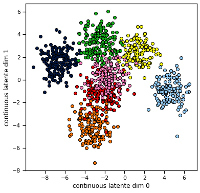
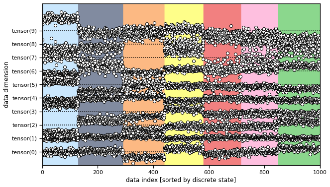
Sample data from the generative model#
Now we will sample small training and testing datasets from an MFA model with random parameters. We plot the data in two ways: as points in the continuous latent space color coded by discrete label, and then as points in the data space. Don’t be fooled by the ordering of the second plot: the samples are arbitrarily ordered, but we’ve permuted their order to see how different states give rise to better see the distribution corresponding to each discrete state.
# Construct a model instance.
# The scale keyword determines how separated the clusters are in the continuous
# latent space.
torch.manual_seed(0)
num_states = 7
latent_dim = 2
data_dim = 10
model = MixtureOfFactorAnalyzers(num_states, latent_dim, data_dim, scale=3)

# Sample from the model
num_data = 1000
train_data = model.sample(sample_shape=(num_data,))
test_data = model.sample(sample_shape=(num_data,))

# Plot the data
model.plot(train_data)
Part 1: Coordinate Ascent Variational Inference (CAVI)#
First, we’ll implement coordinate ascent variational inference (CAVI) for the mixture of factor analyzers model. We’ll use a mean field posterior approximation
such that \(\mathrm{KL}\big( q(z)q(x) \, \| \, p(z, x \mid y, \Theta) \big)\) is minimized. In class, we showed how to minimize the KL via coordinate ascent, iteratively optimizing \(q(z)\) and \(q(x)\), holding the other fixed. Here we will implement that algorithm.
Problem 1a [Math]: Derive the expected log likelihood#
In class we derived the coordinate update for the discrete state factors,
where
However, we did not simplify the expected log likelihood expression.
_Suppose \(q(x_t) = \mathcal{N}(x_t \mid \tilde{\mu}_t, \tilde{\Sigma}_t)\). Show that the expected log likelihood is,
Your answer here
Problem 1b: Implement the discrete state update#
We will use torch.distributions.Distribution objects to represent the approximate posterior distributions as well. We will use MultivariateNormal to represent \(q(x)\) and Categorical to represent \(q(z)\). We’ll take advantage of the distribution objects’ broadcasting capability to represent the variational posteriors for all time steps at once.
Implement a CAVI update for the discrete states posterior that takes in the model and the continuous state posterior q_x and outputs the optimal q_z.
def cavi_update_q_z(model, q_x):
    """Compute the optimal discrete state posterior given the generative model
    and the variational posterior on the continuous states.

    Parameters
    ----------
    model: a MixtureOfFactorAnalyzers model instance.

    q_x: a `MultivariateNormal` object with a shape `TxD` parameter `mean` and a
        shape `TxDxD` parameter `covariance matrix` representing the means and
        covariances, respectively, for each data point under the variational
        posterior.

    Returns
    -------
    q_z: a `Categorical` object with a shape `TxK` parameter `logits`
        representing the variational posterior on discrete states.
    """
    K = model.num_states
    T = q_x.mean.shape[0]

    logits = torch.zeros(T, K)
    ###
    # YOUR CODE BELOW
    for k, (bk, Qk, Jk) in enumerate(zip(model.bs, model.Qs, model.Js)):
        logits[k] += ...
    ###
    return Categorical(logits=logits)
def test_1b():
    torch.manual_seed(0)
    q_x = MultivariateNormal(torch.randn(num_data, latent_dim),
                             torch.eye(latent_dim).repeat(num_data, 1, 1))
    q_z = cavi_update_q_z(model, q_x)
    assert q_z.probs.shape == (num_data, num_states)
    assert torch.isclose(q_z.probs.std(), torch.tensor(0.2576), atol=1e-4)
test_1b()
Problem 1c: Implement the continuous state update#
In class we showed that the optimal continuous state posterior, holding the discrete posterior fixed, was a Gaussian distribution \(q(x_t) = \mathcal{N}(\tilde{\mu}_t, \tilde{\Sigma}_t)\) with
Implement a CAVI update for the continuous states posterior that takes in p_x, p_y, and q_z and outputs the optimal q_x.
def cavi_update_q_x(data, model, q_z):
    """Compute the optimal discrete state posterior given the generative model
    and the variational posterior on the continuous states.

    Parameters
    ----------
    data: a dictionary with a key `y` containing a `TxN` tensor of data.

    model: a MixtureOfFactorAnalyzers model instance.

    q_z: a `Categorical` object with a shape `TxK` parameters `logits` and
        `probs` representing the variational posterior on discrete states.

    Returns
    -------
    q_x: a `MultivariateNormal` object with a shape `TxD` parameter `mean` and a
        shape `TxDxD` parameter `covariance matrix` representing the means and
        covariances, respectively, for each data point under the variational
        posterior.
    """
    y = data["y"]

    ###
    # YOUR CODE BELOW
    q_x = ...
    ###
    return q_x
def test_1c():
    torch.manual_seed(0)
    q_z = Categorical(logits=torch.randn(num_data, num_states))
    q_x = cavi_update_q_x(train_data, model, q_z)
    assert q_x.mean.shape == (num_data, latent_dim)
    assert q_x.covariance_matrix.shape == (num_data, latent_dim, latent_dim)
    assert torch.isclose(q_x.mean.mean(), torch.tensor(-0.7204), atol=1e-4)
    assert torch.isclose(q_x.mean.std(), torch.tensor(2.9253), atol=1e-4)
    assert torch.isclose(q_x.covariance_matrix.mean(), torch.tensor(0.0271), atol=1e-4)
    assert torch.isclose(q_x.covariance_matrix.std(), torch.tensor(0.0623), atol=1e-4)
test_1c()
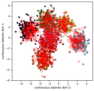
Problem 1d [Short Answer]: Intuition for the continuous updates#
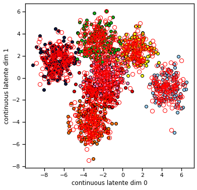
Consider setting the discrete posterior \(q(z)\) to be uniform over the \(K\) states and then performing one update of the continuous states. The plot below shows the true values of \(x\) and \(z\) as color coded dots in 2D, and then it shows the means of the continuous state posterior \(q(x)\) found using one step of CAVI. We see that the means of the continuous state posterior are all pulled toward the center. Why would you expect that to happen?
Your answer here
def plot_data_and_q_x(data, q_x):
    x, z, y = data['x'], data['z'], data['y']
    plt.figure(figsize=(6, 6))
    for k in range(model.num_states):
        plt.plot(x[z == k, 0], x[z == k, 1], 'o', color=palette[k], mec='k')
        plt.plot(q_x.mean[z == k, 0], q_x.mean[z == k, 1], 'o', color=palette[k], mfc='none', mec='r', ms=8)
    plt.xlabel("continuous latente dim 0")
    plt.ylabel("continuous latente dim 1")

q_z = Categorical(logits=torch.zeros(num_data, model.num_states))
q_x = cavi_update_q_x(train_data, model, q_z)
plot_data_and_q_x(train_data, q_x)
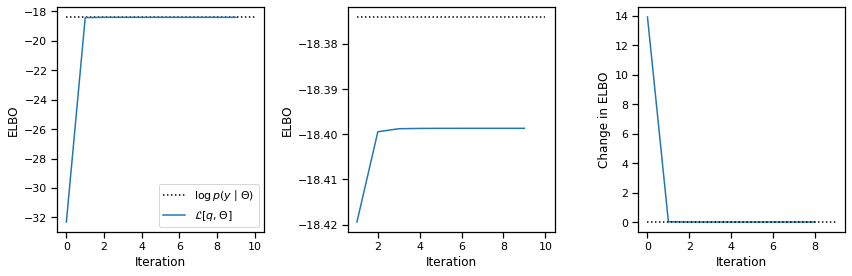
Problem 1e [Math]: Derive the evidence lower bound#
We will use the ELBO to track the convergence of our CAVI algorithm. In class we wrote the ELBO as,
Show that this is equivalent to,
Then show that,
where \(\tilde{\mu}_t\) and \(\tilde{\Sigma}_t\) are the parameters of the variational posterior \(q(x_t)\), as above.
Your answer here
Problem 1f: Implement the ELBO#
Use the IndependentLinearRegression.log_prob function and the torch.distributions.kl_divergence function imported at the top of the notebook to implement the ELBO calculation. Remember that the log probabilities and KL divergence functions broadcast nicely.
def elbo(data, model, variational_posterior):
    """Compute the optimal discrete state posterior given the generative model
    and the variational posterior on the continuous states.

    Parameters
    ----------
    data: a dictionary with a key `y` containing a `TxN` tensor of data.

    model: a MixtureOfFactorAnalyzers model instance

    variational_posterior: a tuple (q_z, q_x) where
        q_z: a `Categorical` object with a shape `TxK` parameter `logits`
            representing the variational posterior on discrete states.

        q_x: a `MultivariateNormal` object with a shape `TxD` parameter `mean`
            and a shape `TxDxD` parameter `covariance matrix` representing the
            means and covariances, respectively, for each data point under the
            variational posterior.

    Returns
    -------
    The evidence lower bound (ELBO) as derived above.
    """
    y = data["y"]
    q_z, q_x = variational_posterior

    ###
    # YOUR CODE BELOW
    elbo = ...
    ###
    return elbo
def test_1f():
    q_z = Categorical(logits=torch.zeros(num_data, model.num_states))
    q_x = cavi_update_q_x(train_data, model, q_z)
    assert torch.isclose(elbo(train_data, model, (q_z, q_x)) / num_data,
                         torch.tensor(-32.3214), atol=1e-4)

test_1f()
Problem 1g [Math]: Derive the exact marginal likelihood#
In this simple model, we can actually compute the marginal likelihood exactly. This gives us a way of seeing how tight the ELBO actually is. (Remember, the ELBO is a lower bound on the marginal likelihood!)
To compute the marginal likelihood, we need two key facts about Gaussian random variables:
Use these two facts to show that
Then show that
Your answer here
Implement the exact marginal likelihood#
The code below implements the exact marginal likelihood according to the formula above using PyTorch’s LowRankMultivariateNormal distribution. Note: this distribution takes in the square root of \(C Q_k C^\top\), which is \(C Q_k^{1/2}\).
def exact_marginal_lkhd(data, model):
    """
    Compute the exact marginal likelihood.
    Normalize by the number of datapoints.
    """
    # Compute the marginal distributions
    y = data["y"]
    T = y.shape[0]
    K = model.num_states

    # Compute the marginal likelihood under each discrete state assignment
    lls = torch.zeros(T, K)
    for k, (bk, Qk) in enumerate(zip(model.bs, model.Qs)):
        # log p(z = k)
        lls[:, k] += model.log_pi[k]

        # logp(y | z = k) = log N(y | C b_k + d, C Q_k C^T + diag(R))
        Qk_sqrt = torch.linalg.cholesky(Qk)
        p_yk = LowRankMultivariateNormal(model.C @ bk + model.d,
                                         model.C @ Qk_sqrt, model.R_diag)
        lls[:, k] += p_yk.log_prob(y)

    return torch.logsumexp(lls, axis=1).sum()

marginal_ll = exact_marginal_lkhd(train_data, model) / num_data
Run CAVI#
That’s all we need for CAVI! The code below simply alternates between updating \(q(z)\) and \(q(x)\). After each iteration, we compute the ELBO.We allow the user to pass in an initial posterior approximation (though only \(q(z)\) is used since \(q(x)\) is immediately updated).
def cavi(data, model, initial_posterior=None, num_steps=10, pbar=None):
    y = data["y"]

    # Initialize the discrete state posterior to uniform
    if initial_posterior is None:
        q_z = Categorical(logits=torch.zeros(len(y), model.num_states))
        q_x = None
    else:
        q_z, _ = initial_posterior

    # Optional progress bar
    if pbar is not None: pbar.reset()

    # Run CAVI
    avg_elbos = []
    for i in range(num_steps):
        if pbar is not None: pbar.update()
        q_x = cavi_update_q_x(data, model, q_z)
        avg_elbos.append(elbo(data, model, (q_z, q_x)) / len(y))
        q_z = cavi_update_q_z(model, q_x)

    return torch.tensor(avg_elbos), (q_z, q_x)
# Run CAVI and plot the ELBO over coordinate ascent iterations
avg_elbos, (q_z, q_x) = cavi(train_data, model)
plot_elbos(avg_elbos, marginal_ll)
Re-examine the continuous state posterior after CAVI#
Now let’s make the same plot from Problem 1d again. We should see that the continuous means are pulled toward their true values. Remember, these are inferences! The CAVI algorithm only sees the data \(y\) and the model parameters \(\Theta\). After a few iterations (really, after about 2 iterations), it converges to a posterior approximation in which the mean of continuous latent states, \(\mathbb{E}_{q(x_t)}[x_t]\), are close to their true values.
plot_data_and_q_x(train_data, q_x)
Part 2: Variational EM in a mixture of factor analysis models#
The CAVI algorithm we implemented in Part 1 will form the E step for variational EM. To complete the algorithm, we just need to compute the expected sufficient statistics under the variational posterior and use them to implement the M-step. Last week, in Lab 7, we derived the expected sufficient statistics needed to update the multivariate normal distribution and the weights of the linear regression. In this part, you’ll write similar functions to compute the expected sufficient statistics using the variational posterior.
Problem 2a: Compute the expected sufficient statistics#
The sufficient statistics of the model are (with zero-indexing for Python friendliness),
\(\sum_{t=1}^T \mathbb{I}[z_t=k]\) for \(k = 1, \ldots, K\)
\(\sum_{t=1}^T \mathbb{I}[z_t=k] \, x_t\) for \(k = 1, \ldots, K\)
\(\sum_{t=1}^T \mathbb{I}[z_t=k] \, x_t x_t^\top\) for \(k = 1, \ldots, K\)
\(\sum_{t=1}^T x_t\)
\(\sum_{t=1}^T x_t x_t^\top\)
\(\sum_{t=1}^T y_t x_t^\top\)
\(\sum_{t=1}^T y_t\)
\(\sum_{t=1}^T y_t^2\)
\(\sum_{t=1}^T 1 = T\)
Write a function that computes the expected sufficient statistics \(\mathbb{E}_{q(z)q(x)}[\cdot]\) under the variational posterior distribution. In code, we’ll call these variables E_*, for example E_z represents the length \(K\) tensor for the sufficient statistic 0.
Note: The expected outer product, \(\mathbb{E}_{q(x_t)}[x_t x_t^\top]\), does not equal the covariance matrix unless \(\mathbb{E}_{q(x_t)}[x_t]\) is zero (and here, it’s not generally zero).
Note: Statistics 3 and 1 are redundant, as are 4 and 2. We’ve split them out anyway, as they are used separately in updating the parameters of p_x and p_y.
def compute_expected_suffstats(data, posterior):
    """
    Compute the expected sufficient statistics of the data
    under the variational posterior

    Parameters
    ----------
    data: a dictionary with a key `y` containing a `TxN` tensor of data.
    posterior: a tuple (q_z, q_x) representing the variational posterior, as
        computed in part 1.

    Returns
    -------
    A tuple of the 9 expected sufficient statistics in the order listed above.
    """
    y = data["y"]
    q_z, q_x = posterior

    E_z = ...
    E_zx = ...
    E_zxxT = ...
    E_x = ...
    E_xxT = ...
    E_yxT = ...
    E_y = ...
    E_ysq = ...
    T = ...
    return (E_z, E_zx, E_zxxT, E_x, E_xxT, E_yxT, E_y, E_ysq, T)
def test_2a():
    print("This test only checks the shapes, not the values!")
    stats = compute_expected_suffstats(train_data, (q_z, q_x))
    assert len(stats) == 9
    E_z, E_zx, E_zxxT, E_x, E_xxT, E_yxT, E_y, E_ysq, T = stats
    assert E_z.shape == (num_states,)
    assert E_zx.shape == (num_states, latent_dim)
    assert E_zxxT.shape == (num_states, latent_dim, latent_dim)
    assert E_x.shape == (latent_dim,)
    assert E_xxT.shape == (latent_dim, latent_dim)
    assert E_yxT.shape == (data_dim, latent_dim)
    assert E_y.shape == (data_dim,)
    assert E_ysq.shape == (data_dim,)
    assert isinstance(T, (int, float))

test_2a()
This test only checks the shapes, not the values!
Problem 2b: Implement the M-step for the parameters of \(p(z \mid \Theta)\)#
Write a function to update the prior distribution on discrete states, \(p(z \mid \Theta)\), using the expected sufficient statistics. This is part of the M-step for variational EM.
def update_p_z(stats):
    """
    Compute the parameters $\pi$ of the $p(z \mid \Theta)$ and pack them into
    a new Categorical distribution object.

    Parameters
    ----------
    stats: a tuple of the 9 sufficient statistics computed above

    Returns
    -------
    A new Categorical object for p_z with a length K tensor of cluster
        probabilities.
    """
    E_z = stats[0]
    ###
    # YOUR CODE BELOW
    p_z = ...
    ###
    return p_z
Problem 2c: Implement the M-step for parameters of \(p(x \mid z, \Theta)\)#
Perform an M-step on the parameters of \(p(x \mid z, \Theta)\) using the expected sufficient statistics. As before, add a little to the diagonal of the covariance to ensure positive definiteness.
def update_p_x(stats):
    """
    Compute the parameters $\{b_k, Q_k\}$ of the $p(x \mid z, \Theta)$ and pack
    them into a new MultivariateNormal distribution object.

    Parameters
    ----------
    stats: a tuple of the 9 sufficient statistics computed above

    Returns
    -------
    A new MultivariateNormal object with KxD mean and KxDxD covariance matrix.
    """
    E_z, E_zx, E_zxxT = stats[:3]
    K, D = E_zx.shape

    ###
    # YOUR CODE BELOW
    p_x = ...
    #
    ###
    return p_x
Problem 2d: Implement the M-step for parameters of \(p(y \mid x, \Theta)\)#
Following Lab 7, let \(\phi_t = (x_t, 1)\) denote the covariates that go into the linear model for data point \(y_t\). Specifically,
where \(W = (C, d) \in \mathbb{R}^{N \times D+1}\) is an array containing both the weights and the bias of the linear regression model.
To update the linear regression, we need the expected sufficient statistics:
The expected outer product of the data and covariates,
The expected outer product of the covariates with themselves,
These are \(N \times (D+1)\) and \((D+1) \times (D+1)\) tensors, respectively.
Since we are assuming a diagonal covariance matrix, we only need \(y_{tn}^2\) instead of the full outer product \(y_t y_t^\top\). As before, add a bit to the diagonal to ensure positive definiteness.
def update_p_y(stats):
    """
    Compute the linear regression parameters given the expected
    sufficient statistics.

    Note: add a little bit to the diagonal of each covariance
        matrix to ensure that the result is positive definite.

    Parameters
    ----------
    stats: a tuple of the 8 sufficient statistics computed above

    Returns
    -------
    A new IndependentLinearRegression object for p_y
    """
    E_x, E_xxT, E_yxT, E_y, E_ysq, T = stats[3:]
    N, D = E_yxT.shape

    ###
    # Use E_x, E_xxT, E_yxT, E_y, and T to compute the full expected
    # sufficient matrices as described above.
    #
    # YOUR CODE BELOE
    p_y = ...
    #
    ###

    return p_y
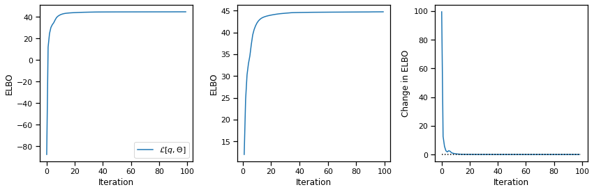
Put it all together#
From here it’s smooth sailing! We just iterate between the variational E step, which involves running CAVI for some number of iterations, and then performing an M step using expected sufficient statistics. We’ll track the ELBO throughout to monitor convergence.
def m_step(data, model, posterior):
    """
    Perform an M-step to update the model parameters given the data and the
    posterior from the variational E step.
    """
    stats = compute_expected_suffstats(data, posterior)
    model.p_z = update_p_z(stats)
    model.p_x = update_p_x(stats)
    model.p_y = update_p_y(stats)


def variational_em(data, model, num_iters=100, num_cavi_steps=1):
    """
    Fit the model parameters via variational EM.
    """
    # Run CAVI
    avg_elbos = []
    posterior = None
    for i in trange(num_iters):
        # Variational E step with CAVI
        these_elbos, posterior = cavi(data, model, posterior,
                                      num_steps=num_cavi_steps)
        avg_elbos.extend(these_elbos)

        # M-step
        m_step(data, model, posterior)

    return torch.tensor(avg_elbos), posterior
# Fit the synthetic data
avg_elbos, posterior = variational_em(train_data, model)
plot_elbos(avg_elbos, marginal_ll)
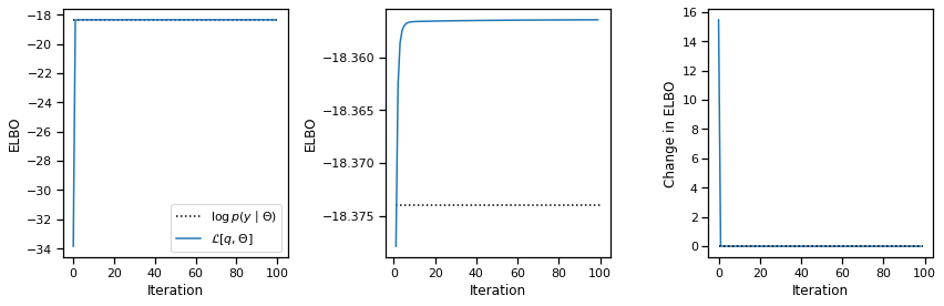
Problem 2e [Short Answer]: Interpret the results#
One perhaps counterintuitive aspect of the output is that the ELBO of the fitted model actually exceeds the marginal likeliood of the true model. How can that happen?
Answer below this line
Problem 2f: Cross validation#
Fit the MFA model with variational EM for \(D=1,\ldots, 5\) (inclusive), keeping the number of discrete states fixed to \(K=7\). For each model, evaluate the evidence lower bound on the test data, using ten steps of CAVI to approximate the posterior. Then compute the exact marginal likelihood using the true model and compare.
test_latent_dims = torch.arange(1, 11)
test_elbos = []
for d in test_latent_dims:
    print("Fitting the MFA model with D =", int(d),
          "dimensional continuous states.")
    ###
    # YOUR CODE BELOW
    # ...
    test_elbos.append(...)
    #
    ###

# Compute the true marginal likelihood of the test dat
true_test_elbo = exact_marginal_lkhd(test_data, model) / num_data

# Plot as a function of continuous dimensionality
plt.plot(test_latent_dims, test_elbos, '-o')
plt.plot(test_latent_dims, true_test_elbo * torch.ones_like(test_latent_dims), ':k')
plt.xlabel("continuous dimension $D$")
plt.ylabel("Test ELBO")
Fitting the MFA model with D = 1 dimensional continuous states.
Fitting the MFA model with D = 2 dimensional continuous states.
Fitting the MFA model with D = 3 dimensional continuous states.
Fitting the MFA model with D = 4 dimensional continuous states.
Fitting the MFA model with D = 5 dimensional continuous states.
Fitting the MFA model with D = 6 dimensional continuous states.
Fitting the MFA model with D = 7 dimensional continuous states.
Fitting the MFA model with D = 8 dimensional continuous states.
Fitting the MFA model with D = 9 dimensional continuous states.
Fitting the MFA model with D = 10 dimensional continuous states.
Text(0, 0.5, 'Test ELBO')
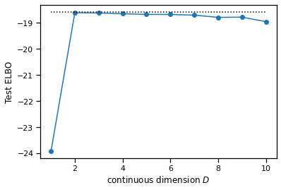
Problem 2g [Short answer]: Interpret the results#
Would you be surprised to see the fitted models achieve higher ELBOs on test data than the marginal likelihod of the true model? Can you think of any potential concerns with using the ELBO for model comparison; e.g. for selecting the latent state dimension \(D\)?
Your answer here
Part 3: Apply it to real data#
Finally, we’ll apply the mixture of factor analyzers to calcium imaging data from immobilized worms studied by Kato et al (2015). They also segmented the time series into discrete states based on the neural activity and gave each state a name, using their knowledge of how different neurons correlate with different types of behavior. We’ll try to recapitulate some of their results using the MFA model to infer discrete states.
%%capture
!wget -nc https://www.dropbox.com/s/qnjslekm11pyuju/kato2015.zip
!unzip -n kato2015.zip
Load the data#
The data is stored in a dictionary with a few extra keys for the neuron names and the given discrete state labels and human-interpretable state names.
# Load the data for a single worm
data = load_kato(index=4)

# Extract key constants
num_frames, num_neurons = data["y"].shape
times = torch.arange(num_frames) / data["fps"]

print(data.keys())
dict_keys(['neuron_names', 'y', 'z_kato', 'state_names', 'fps'])
Perform PCA#
We’ll use the principal components for visualization as well as for finding a permutation of the neurons that puts similar neurons, as measured by their loading on the first principal component, near to one another.
# Perform PCA
pca = PCA(20)
data["pcs"] = pca.fit_transform(data["y"])
neuron_perm = torch.argsort(torch.tensor(pca.components_[0]))
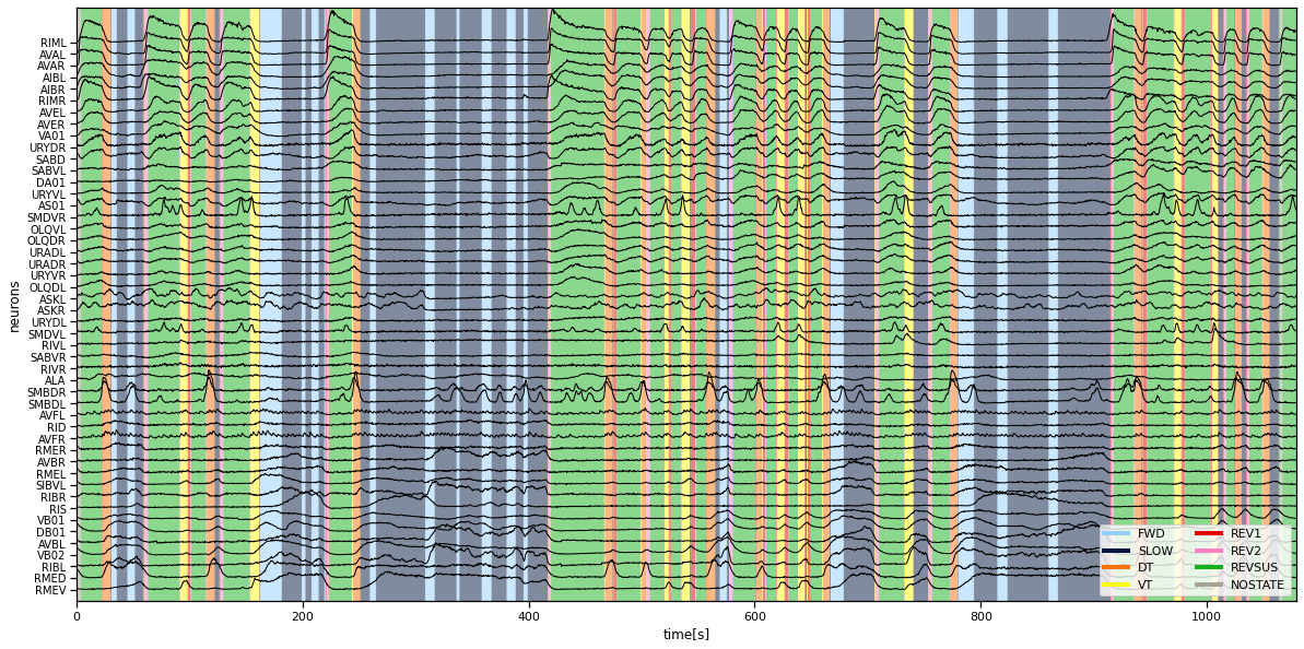
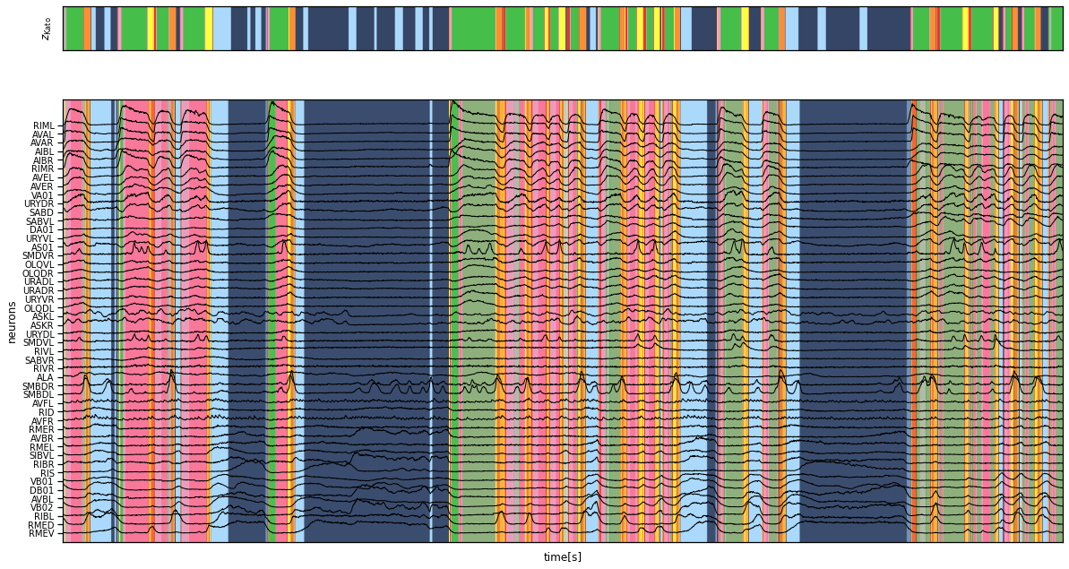
Plot the data#
We plot the time series of neural activity on top of the color-coded discrete states given by Kato et al. You should see that the different discrete states correspond to different levels of neural activity across the population of neurons.
plt.figure(figsize=(20, 10))
plt.imshow(data["z_kato"][None, :], extent=(0, times[-1], -1, num_neurons + 2),
           alpha=0.5, cmap=cmap, aspect="auto")
plt.plot(times, data["y"][:, neuron_perm] + torch.arange(num_neurons), '-k', lw=1)
plt.xlabel("time[s]")
plt.ylabel("neurons")
plt.yticks(torch.arange(num_neurons),
           [data["neuron_names"][i] for i in neuron_perm],
           fontsize=10)
plt.ylim(-1, num_neurons+2)

for state_name, color in zip(data["state_names"], palette):
    plt.plot([torch.nan], [torch.nan], '-', color=color, lw=4, label=state_name)

plt.legend(loc="lower right", ncol=2)
<matplotlib.legend.Legend at 0x7f414c9e73d0>
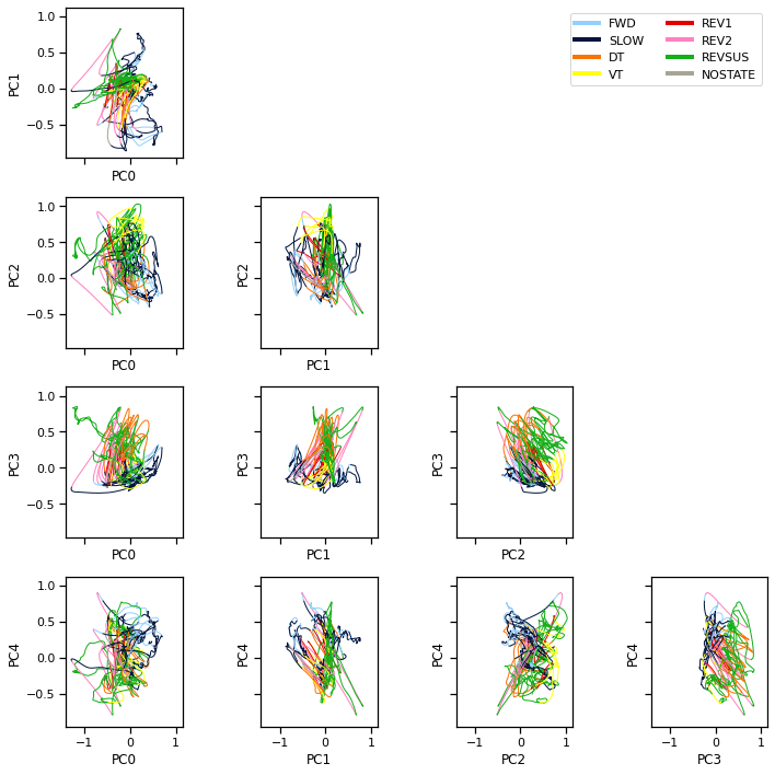
Plot the PCA trajectories#
We can also visualize the population activity as a trajectory through PCA space. Here we plot the trajectory in planes spanned by pairs of principal components. We color code the trajectory based on the given discrete states.
Note: We smoothed the trajectories a bit to make the visualization nicer.
Note: These differ from the figures in Kato et al (2015) in that they used PCA on the first order differences in neural activity (akin to the “spikes” in the calcium trace, even though C elegans doesn’t fire action potentials). We found that the first order differences didn’t cluster as nicely with the MFA model, so we are working with the calcium traces directly.
pcs_smooth = gaussian_filter1d(data["pcs"], 1, axis=0)

fig, axs = plt.subplots(4, 4, figsize=(10, 10), sharex=True, sharey=True)
for i in range(4):
    for j in range(i+1, 5):
        plot_2d_continuous_states(pcs_smooth, data["z_kato"],
                                  ax=axs[j-1, i], inds=(i, j), lw=1)
        axs[j-1, i].set_xlabel("PC{}".format(i))
        axs[j-1, i].set_ylabel("PC{}".format(j))

    for j in range(i):
        axs[j, i].set_axis_off()

for state_name, color in zip(data["state_names"], palette):
    axs[0, -1].plot([torch.nan], [torch.nan], '-',
                    color=color, lw=4, label=state_name)
axs[0, -1].legend(loc="upper right", ncol=2, )

plt.tight_layout()
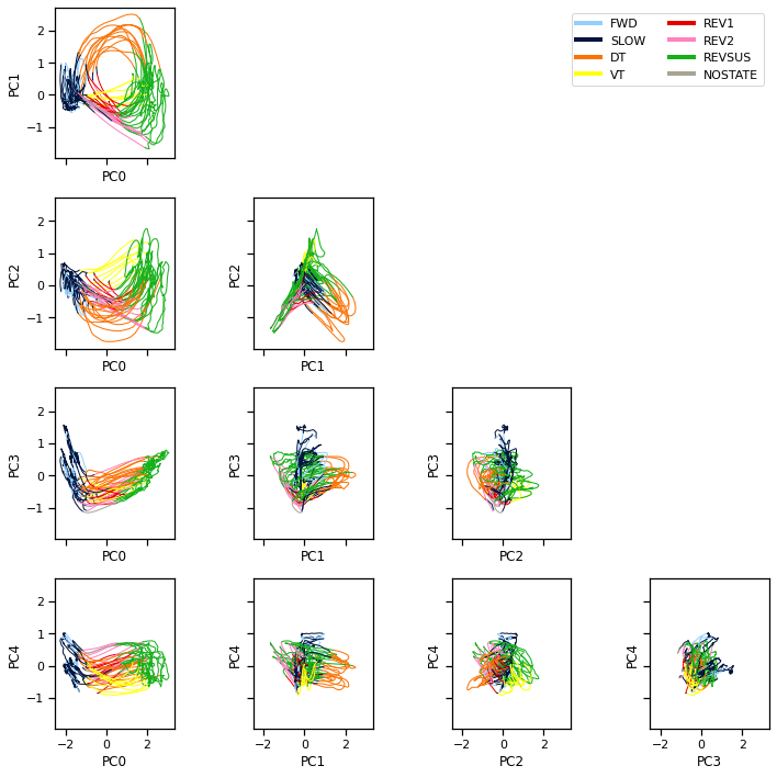
Problem 3a [Short Answer]: Interpret the PCA trajectories#
What can you say about the cycle of neural activity in this worm given the PCA trajectories and the state labels provided by Kato et al (2015)?
Answer below this line
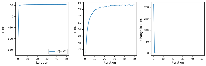
Fit the mixture of factor analyzers#
Now fit the model. We’ll give it twice as many states as Kato et al (2015) did. This often helps avoid some local optima where states are unused. We’ll use ten dimensional continuous latents, as they do in the paper.
# Fit the worm data
torch.manual_seed(0)
num_states = 16
latent_dim = 10
worm_model = MixtureOfFactorAnalyzers(num_states, latent_dim, num_neurons)

# Fit the model!
avg_elbos, posterior = variational_em(data, worm_model,
                                      num_iters=100,
                                      num_cavi_steps=1)

plot_elbos(avg_elbos)
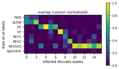
Compute the overlap between the given and inferred discrete states#
# Find the most likely state segmentation
q_z, q_x = posterior
z_inf = q_z.probs.argmax(axis=1)

# compute overlap with the manually labeled states
overlap = torch.zeros(8, num_states)
for i in range(8):
    for j in range(num_states):
        overlap[i, j] = torch.sum((data["z_kato"] == i) * (z_inf == j))

# normalize since sum given states are used less frequently than others
overlap /= overlap.sum(axis=0)

# permute the inferred labels for easier visualization
z_perm = torch.argsort(torch.argmax(overlap, axis=0))

# show the permuted overlap matrix
plt.imshow(overlap[:, z_perm])
plt.ylabel("Kato et al labels")
plt.yticks(torch.arange(8), data["state_names"])
plt.xlabel("inferred discrete states")
plt.title("overlap (column normalized)")
plt.colorbar()

# Permute the inferred discrete states per the new ordering
z_inf_perm = torch.argsort(z_perm)[z_inf]
Plot the inferred segmentation and the given state labels#
fig, axs = plt.subplots(2, 1, figsize=(20, 11),
                        gridspec_kw=dict(height_ratios=[1, 10]),
                        sharex=True)

axs[0].imshow(data["z_kato"][None, :],
              extent=(0, times[-1], 0, 1),
              alpha=0.8, cmap=cmap, aspect="auto")
axs[0].set_xticks([])
axs[0].set_yticks([])
axs[0].set_ylabel("$z_{\mathsf{Kato}}$")

axs[1].imshow(z_inf_perm[None, :], extent=(0, times[-1], -1, num_neurons + 2),
              cmap=cmap, alpha=0.8, aspect="auto")
axs[1].plot(times, data["y"][:, neuron_perm] + torch.arange(num_neurons),
            '-k', lw=1)
axs[1].set_xlabel("time[s]")
axs[1].set_yticks(torch.arange(num_neurons))
axs[1].set_yticklabels([data["neuron_names"][i] for i in neuron_perm],
                       fontsize=10)
axs[1].set_ylabel("neurons")
axs[1].set_ylim(-1, num_neurons+2)
(-1.0, 50.0)
x_inf = q_x.mean
x_inf_smooth = gaussian_filter1d(x_inf, 2, axis=0)

fig, axs = plt.subplots(4, 4, figsize=(10, 10), sharex=True, sharey=True)
for i in range(4):
    for j in range(i+1, 5):
        plot_2d_continuous_states(x_inf_smooth, data["z_kato"],
                                  ax=axs[j-1, i], inds=(i, j), lw=1)
        axs[j-1, i].set_xlabel("PC{}".format(i))
        axs[j-1, i].set_ylabel("PC{}".format(j))

    for j in range(i):
        axs[j, i].set_axis_off()

for state_name, color in zip(data["state_names"], palette):
    axs[0, -1].plot([torch.nan], [torch.nan], '-',
                    color=color, lw=4, label=state_name)
axs[0, -1].legend(loc="upper right", ncol=2, )

plt.tight_layout()
Bonus: Problem 3b: Compare and contrast#
We fit the model with twice as many discrete states as Kato et al (2015) reported. Split this time series into training and test sets and then sweep over \(K\) to choose the number of discrete states by cross validation.
Write your analysis code in the cell below and describe your results in words below this line
###
#
# YOUR ANALYSIS CODE BELOW

#
###
Bonus: Problem 3c: Assessing variability across initializations#
The estimated parameters and the inferred posterior depend on the random intialization of the model. How much does that affect our results? To compare the segmentations across model fits, make a \(T \times T\) matrix that shows how often the most likely discrete state at time \(t\) is the same as that at time \(t'\). I.e. let \(\hat{z}_t^{(i)} = \mathrm{argmax}_k q(z_{t}^{(i)}=k)\), where the superscript \((i)\) denotes inferred posterior from the \(i\)-th model fit. Make a matrix whose entries are the average of the indicator \(\mathbb{I}[\hat{z}_t^{(i)} = \hat{z}_{t'}^{(i)}]\) taken over multiple fits of the MFA model with different random initializations.
###
#
# YOUR ANALYSIS CODE BELOW

#
###
Part 4: Switching Linear Dynamical Systems (SLDS)#
If you’re interested in digging deeper and fitting models that explicitly incorporate temporal dependencies, check out the SSM package! To get you started, here’s some code to start fitting SLDS to this dataset.
Note that by default SSM uses a Laplace approximation for the continuous state posterior, which it fits with Newton’s method. Likewise, it uses a Monte Carlo approximation for the M-step, which works with non-Gaussian observation models. For the special case of Gaussian observations, we could find the exact posterior update for \(q(x_{1:T})\) and exact M-steps, as described in class. That would be a bit faster than the code below, but this is still fast enough for our purposes.
For more information, check out the demo notebooks!
Finally, you might also be interested in our latest project, Dynamax, which has JAX implementations of many probabilistic state space models. (Unfortunately, not yet SLDS!)
try:
    import ssm
except:
    !pip install git+https://github.com/lindermanlab/ssm.git@master#egg=ssm

from ssm import SLDS
slds = SLDS(num_neurons, num_states, latent_dim)
elbos, posterior = slds.fit(from_t(data["y"]), num_iters=50)

# Plot the normalized elbos
plot_elbos(elbos / num_frames)
Looking in indexes: https://pypi.org/simple, https://us-python.pkg.dev/colab-wheels/public/simple/
Collecting ssm
  Cloning https://github.com/lindermanlab/ssm.git (to revision master) to /tmp/pip-install-v40s2lyd/ssm_7022d754fa2d40199508dd4c4fc7d9b1
  Running command git clone --filter=blob:none --quiet https://github.com/lindermanlab/ssm.git /tmp/pip-install-v40s2lyd/ssm_7022d754fa2d40199508dd4c4fc7d9b1
  Resolved https://github.com/lindermanlab/ssm.git to commit 6c856ad3967941d176eb348bcd490cfaaa08ba60
  Preparing metadata (setup.py) ... ?25l?25hdone
Requirement already satisfied: numpy>=1.18 in /usr/local/lib/python3.8/dist-packages (from ssm) (1.22.4)
Requirement already satisfied: scipy in /usr/local/lib/python3.8/dist-packages (from ssm) (1.10.1)
Requirement already satisfied: numba in /usr/local/lib/python3.8/dist-packages (from ssm) (0.56.4)
Requirement already satisfied: scikit-learn in /usr/local/lib/python3.8/dist-packages (from ssm) (1.2.1)
Requirement already satisfied: tqdm in /usr/local/lib/python3.8/dist-packages (from ssm) (4.64.1)
Requirement already satisfied: autograd in /usr/local/lib/python3.8/dist-packages (from ssm) (1.5)
Requirement already satisfied: cython in /usr/local/lib/python3.8/dist-packages (from ssm) (0.29.33)
Requirement already satisfied: future>=0.15.2 in /usr/local/lib/python3.8/dist-packages (from autograd->ssm) (0.16.0)
Requirement already satisfied: importlib-metadata in /usr/local/lib/python3.8/dist-packages (from numba->ssm) (6.0.0)
Requirement already satisfied: llvmlite<0.40,>=0.39.0dev0 in /usr/local/lib/python3.8/dist-packages (from numba->ssm) (0.39.1)
Requirement already satisfied: setuptools in /usr/local/lib/python3.8/dist-packages (from numba->ssm) (57.4.0)
Requirement already satisfied: threadpoolctl>=2.0.0 in /usr/local/lib/python3.8/dist-packages (from scikit-learn->ssm) (3.1.0)
Requirement already satisfied: joblib>=1.1.1 in /usr/local/lib/python3.8/dist-packages (from scikit-learn->ssm) (1.2.0)
Requirement already satisfied: zipp>=0.5 in /usr/local/lib/python3.8/dist-packages (from importlib-metadata->numba->ssm) (3.15.0)
Building wheels for collected packages: ssm
  Building wheel for ssm (setup.py) ... ?25l?25hdone
  Created wheel for ssm: filename=ssm-0.0.1-cp38-cp38-linux_x86_64.whl size=562291 sha256=dd86a3a39db8d1948fa3d7685783a081cb71b5f55d899f1d886b0ad38f1c32e0
  Stored in directory: /tmp/pip-ephem-wheel-cache-zqgxan2j/wheels/50/34/75/a5397844576e080cdc001e6421017d9f4e355f83a1dd23f481
Successfully built ssm
Installing collected packages: ssm
Successfully installed ssm-0.0.1
Initializing with an ARHMM using 25 steps of EM.
Submission Instructions#
Formatting: check that your code does not exceed 80 characters in line width. You can set Tools → Settings → Editor → Vertical ruler column to 80 to see when you’ve exceeded the limit.
Download your notebook in .ipynb format and use the following commands to convert it to PDF.
Option 1 (best case): ipynb → pdf Run the following command to convert to a PDF:
jupyter nbconvert --to pdf lab7_teamname.ipynb
Unfortunately, nbconvert sometimes crashes with long notebooks. If that happens, here are a few options:
Option 2 (next best): ipynb → tex → pdf:
jupyter nbconvert --to latex lab7_teamname.ipynb
pdflatex lab7_teamname.tex
Option 3: ipynb → html → pdf:
jupyter nbconvert --to html lab7_teamname.ipynb
# open lab7_teamname.html in browser and print to pdf
Dependencies:
nbconvert: If you’re using Anaconda for package management,
conda install -c anaconda nbconvert
pdflatex: It comes with standard TeX distributions like TeXLive, MacTex, etc. Alternatively, you can upload the .tex and supporting files to Overleaf (free with Stanford address) and use it to compile to pdf.
Upload your .ipynb and .pdf files to Gradescope.
Only one submission per team!