Probabilistic Modeling#
Probabilistic models are distributions over data. The shape of the distribution is determine by model parameters. Our goal to estimate or infer those parameters from observed data.
As the course goes on, we will encounter more and more complex datasets, and we will construct more and more sophisticated models. However, our models will still be composed of just a handful of basic building blocks, and our central goal of parameter estimation and inference remains the same.
Slides for this chapter can be downloaded here.
Simple example#
For example, let \(x_t \in \mathbb{N}_0\) denote the number of spikes a neuron fires in time bin \(t\). One of the simplest (and yet surprisingly not bad) models of neural spike counts is the Poisson distribution with rate \(\lambda \in \mathbb{R}_+\),
The Poisson distribution has a simple probability mass function (pmf),
For Poisson random variables, the mean, aka expected value, \(\mathbb{E}[x_t]\), and variance, \(\mathbb{V}[x_t]\), are both equal to \(\lambda\).
Notation
\(x_t \in \mathbb{N}_0\) means that the variable \(x_t\) is in (\(\in\)) the set \(\mathbb{N}_0\), which is shorthand for the non-negative integers,
\(\lambda \in \mathbb{R}_+\) means that the rate \(\lambda\) is a non-negative real number.
Notation
The first equation says that the spike count \(x_t\) is a random variable whose distribution is (\(\sim\)) Poisson with rate \(\lambda\).
In the second equation, \(\mathrm{Pois}(x_t; \lambda)\) refers to the pmf of the Poisson distribution evaluated at the point \(x_t\). The notation can be a little confusing at first, but it’s a standard convention.
Sampling from a Poisson distribution#
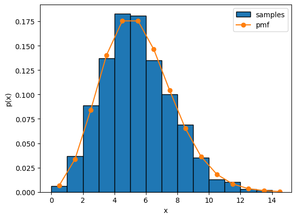
Expand the code below to see how to sample a Poisson distribution using the torch.distributions.Poisson object in PyTorch. The code plots the empirical distribution of 1000 independent samples from the Poisson distribution alongside the Poisson pmf.
Show code cell source
import torch
from torch.distributions import Poisson
import matplotlib.pyplot as plt

# Construct a Poisson distribution with rate 5.0 and draw 1000 samples
rate = 5.0
pois = Poisson(rate)
xs = pois.sample(sample_shape=(1000,))

# Plot a histogram of the samples and overlay the pmf
bins = torch.arange(15)
plt.hist(xs, bins, density=True, edgecolor='k', label='samples')
plt.plot(bins + .5, torch.exp(pois.log_prob(bins)), '-o', label='pmf')
plt.xlabel("x")
plt.ylabel("p(x)")
_ = plt.legend()
/opt/hostedtoolcache/Python/3.9.16/x64/lib/python3.9/site-packages/tqdm/auto.py:21: TqdmWarning: IProgress not found. Please update jupyter and ipywidgets. See https://ipywidgets.readthedocs.io/en/stable/user_install.html
  from .autonotebook import tqdm as notebook_tqdm
Fitting a Poisson distribution#
Now suppose you observe the empirical spike counts sampled above (i.e. the blue histogram) and you want to estimate the rate \(\lambda\).
Let \(\mathbf{x} = (x_1, \ldots, x_T)\) denote the vector of spike counts.
Since the simulated spike counts are independent random variables, their joint probability is a product of Poisson pmf’s,
We want to find the rate that maximizes this probability,
This is called maximum likelihood estimation, and \(\lambda_{\mathsf{MLE}}\) is called the maximum likelihood estimate (MLE).
Solving for the MLE#
In this simple model, we can derive a closed form expression for the MLE.
First, note that maximizing \(p(\mathbf{x}; \lambda)\) is the same as maximizing \(\log p(\mathbf{x}; \lambda)\), since the log is a concave function.
Taking logs of both sides, we find
To maximize with respect to \(\lambda\), we simply take the derivative, set it to zero, and solve for \(\lambda\),
Setting to zero and solving yields,
In other words, the MLE is just the mean of the empirical spike counts, which seems sensible!
Adding a prior distribution#
Maximum likelihood estimation finds the rate that maximizes the probability of the observed spike counts, but it doesn’t take into account any prior information.
For example, this may not be the first neuron you’ve ever encountered. Maybe, based on your experience, you have a sense for the distribution of neural firing rates. That knowledge can be encoded in a prior distribution.
One common choice of prior on rates is the gamma distribution,
The gamma distribution has support for \(\lambda \in \mathbb{R}_+\), and it is governed by two parameters:
\(\alpha\), the shape or concentration parameter, and
\(\beta\), the inverse scale or rate parameter.
It’s probability density function (pdf) is,
where \(\Gamma(\cdot)\) denotes the gamma function.
PDFs vs PMFs
Since the gamma distribution has continuous support over the non-negative reals as opposed to discrete support over, say, the non-negative integers, it has a probability density function rather than a probability mass function.
Technically, the probability that \(\lambda\) falls in a subset of \(\mathbb{R}_+\), like the interval \([a, b)\), is the integral of the probability density function,
Sampling from a gamma distribution#
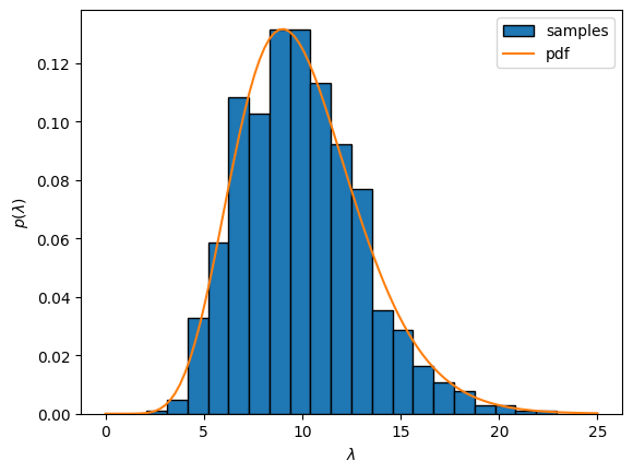
Expand the code below to see how to sample a gamma distribution using the torch.distributions.Gamma object. The code plots the empirical distribution of 1000 independent samples from the gamma distribution, binned into 25 evenly sized bins. It overlays the gamma pdf for comparison.
In words, we might say this particular gamma distribution conveys a prior belief that
Firing rates are usually around 10 spikes/time bin with standard deviation of around 3 spikes/time bin.
Show code cell source
import torch
from torch.distributions import Gamma
import matplotlib.pyplot as plt

# Construct a gamma distribution
alpha = 10.0
beta = 10.0/10.0
gam = Gamma(alpha, beta)
lambdas = gam.sample(sample_shape=(1000,))

# Plot a histogram of the samples and overlay the pmf
grid = torch.linspace(0, 25, 100)
bins = torch.linspace(0, 25, 25)
plt.hist(lambdas, bins, density=True, edgecolor='k', label='samples')
plt.plot(grid, torch.exp(gam.log_prob(grid)), '-', label='pdf')
plt.xlabel(r"$\lambda$")
plt.ylabel(r"$p(\lambda)$")
_ = plt.legend()
Fitting a Poisson distribution with a gamma prior#
When we add in the prior distribution on \(\lambda\), it becomes a random variable too. Now we have to consider the joint distribution of \(\mathbf{x}\) and \(\lambda\),
Warning
We dropped the dependence on the parameters of the gamma prior, \(\alpha\) and \(\beta\). Technically, we should write \(p(\mathbf{x}, \lambda; \alpha, \beta)\), but that gets cumbersome.
The Product Rule, the Sum Rule, and Bayes’ Rule
In the first line we applied the product rule of probability, which says that we can rewrite a joint distribution as a product of a marginal distribution and a conditional distribution
The order doesn’t matter; we could alternatively write,
The marginal distributions \(p(x)\) and \(p(y)\) are obtained via the sum rule,
where \(\mathcal{Y}\) is the support of the random variable \(y\).
Finally, putting both together, we obtain Bayes’ rule,
Bars vs semicolons
Why do we sometimes use bars (\(\mid\)) and other times semicolons (;)? Technically, we use the bar when we are writing a conditional distribution of one random variable given another, like \(p(x \mid y)\) in Bayes’ rule above. When we simply want to write a function that depends on some parameters, we use a semicolon, like \(p(x; \theta)\).
So why did we switch from writing \(p(\mathbf{x}; \lambda)\) to \(p(\mathbf{x} \mid \lambda)\)? Because when we placed a prior on \(\lambda\), we switched from treating \(\lambda\) as a parameter to instead thinking of it as a random variable. It’s a technical distinction, but we’ll try to be precise!
Bayesian inference#
What does it mean to “fit” the rate of a Poisson distribution under a gamma prior? Formally, we perform Bayesian inference.
We want to compute the posterior distribution of the rate \(\lambda\) given the observed spike counts \(\mathbf{x}\) (and the prior parameters \(\alpha\) and \(\beta\), which are assumed fixed),
By Bayes’ rule (see box above), the posterior distribution is equal to the ratio of the joint distribution over the marginal distribution,
Note that the denominator (the marginal distribution) does not depend on \(\lambda\), so the posterior is proportional to the joint,
Maximum a posteriori inference#
A simple summary of the posterior distribution is its mode — the point(s) where the pdf is maximized,
or equivalently,
since the posterior is proportional to the joint.
Warning
True Bayesians cringe at MAP estimation! How can a single point (the mode) summarize an entire distribution!? It can’t, but we’ll use it for now and be better Bayesians later in the course.
Conjugate priors#
Now let’s go back and expand the Poisson pmf and the gamma pdf in the joint distribution,
Many of these terms can be combined! After simplifying,
where
and \(C\) is a constant with respect to \(\lambda\).
Thus, the posterior distribution is a gamma distribution, just like the prior! For this reason, we say the gamma is a conjugate prior for the rate of the Poisson distribution.
Solving for the MAP estimate#
How do we solve for the MAP estimate, \(\lambda_{\mathsf{MAP}} = \text{arg max} \; p(\lambda \mid \mathbf{x})\)?
Now that you know the posterior is a gamma distribution, you can expand its pdf, take the log, take the derivative wrt \(\lambda\), set it to zero and solve.
Or you can just go to the Wikipedia page on the gamma distribution and see that its mode is
for \(\alpha' \geq 1\), and 0 otherwise.
Uninformative priors
When does the MAP estimate coincide with the MLE? Intuitively, that happens when the prior probability is flat, or uninformative. Unfortunately, it’s impossible to have a flat prior over the entire set of non-negative reals since the pdf has to integrate to one. However, we obtain an uninformative gamma prior in the limit that \(\alpha \to 1\) and \(\beta \to 0\). In that limit, \(\alpha' \to \sum_t x_t\) and \(\beta' \to T\) so that \(\lambda_{\mathsf{MAP}} \to \frac{1}{T} \sum_t x_t = \lambda_{\mathsf{MLE}}\).
MAP estimation in our simulated example#
Take the simulated data from above. What is the MAP estimate of the rate given the observed spike counts and the prior, and how does it compare to the MLE? We have…
alpha_post = alpha + xs.sum()
beta_post = beta + len(xs)

lambda_mle = xs.sum() / len(xs)
lambda_map = (alpha_post - 1) / beta_post

print("MLE:", lambda_mle)
print("MAP:", lambda_map)
MLE: tensor(4.9420)
MAP: tensor(4.9461)
Questions
Why is the MAP estimate slightly higher than the MLE?
What if you make \(T\) smaller? Change the code above to sample \(20\) spike counts instead of 1000. How does that change the MAP/MLE difference?
Mixture models and latent variables#
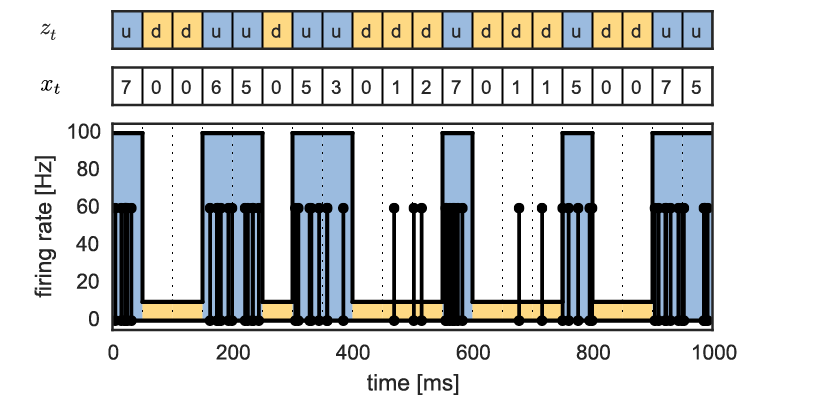
Fig. 1 Example of a mixture model with a latent variable \(z_t\) specifying whether the neuron is in the up or down state.#
We’ve already gotten a lot of mileage out of this simple Poisson example! However, real data will rarely be so simple. One way to build richer models is by introducing latent variables.
For example, suppose that at each time bin \(t\), the neuron can either be in an up state with a high firing rate, or a down state with low firing rate.
Let \(z_t \in \{0,1\}\) be a latent variable (something we don’t explicitly observe) that denotes which state the neuron in is at that time, with 1 meaning up and 0 meaning down. Likewise, let \(\lambda_1\) and \(\lambda_0\) denote the corresponding firing rates, with \(\lambda_1 > \lambda_0\).
We will place gamma priors the firing rates, \(\lambda_1 \sim \mathrm{Ga}(\alpha, \beta)\) and \(\lambda_0 \sim \mathrm{Ga}(\alpha, \beta)\). (We could get fancy here, but let’s keep it simple for now.)
Finally, assume that the latent variables are equally probable and independent across time. Formally, we can write that as a categorical distribution with equal probabilities for both states,
The resulting model is called a mixture model because the marginal distribution, \(p(x_t \mid \boldsymbol{\lambda})\) where \(\boldsymbol{\lambda} = (\lambda_0, \lambda_1)\), is a mixture of two Poisson distributions,
Question
What probability rule did we use to get this marginal distribution?
Sampling a Poisson mixture model#
Let’s draw samples from the mixture model, like we did above for the single Poisson distribution.
Show code cell source
import torch
from torch.distributions import Poisson, Categorical
import matplotlib.pyplot as plt

# Construct a Poisson mixture model with down rate 1.0 and up rate 10.0
rates = torch.asarray([1.0, 10.0])
cat = Categorical(torch.asarray([0.5, 0.5]))
T = 1000

# Sample the states from the categorical distribution
zs = cat.sample(sample_shape=(T,))

# Sample the spike counts from a Poisson distribution
# using the rate for the corresponding state.
# Note: this uses PyTorch's broadcasting semantics.
xs = Poisson(rates[zs]).sample()

# Compute the mixture probability at a range of bins
bins = torch.arange(20)
up_pmf = torch.exp(Poisson(rates[1]).log_prob(bins))
down_pmf = torch.exp(Poisson(rates[0]).log_prob(bins))
mixture_pmf = 0.5 * (up_pmf + down_pmf)

# Plot a histogram of the samples and overlay the pmf
plt.hist(xs, bins, density=True, edgecolor='k', label='samples')
plt.plot(bins + 0.5, mixture_pmf, '-o', label='pmf')
plt.xlabel("x")
plt.ylabel("p(x)")
_ = plt.legend()
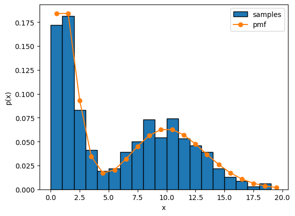
With this model, we can capture multimodal firing rate distributions.
The MixtureSameFamily class
We manually sampled the mixture distribution by first sampling the Categorical and then the Poisson. PyTorch also provides a MixtureSameFamily class to do this in one step.
Fitting a mixture model by coordinate ascent#
Conceptually, fitting the mixture model is no different than fitting the the simple Poisson model above.
We will perform MAP estimation to find,
where \(\mathbf{z} = (z_1, \ldots, z_T)\). Again, this is equivalent to maximizing the joint probability.
Expanding the joint distribution over spike counts, latent variables, and rates,
Our strategy for maximizing this objective is to iteratively maximize with respect to one variable at a time, holding the rest fixed. This is called coordinate ascent.
Fixing the rates, the most likely state at time \(t\) is,
Fixing the states, the most likely rates are
for \(k \in \{0, 1\}\).
Notation
The indicator function \(\mathbb{I}[y]\) equals 1 if the predicate \(y\) is true; otherwise it equals zero.
Exercise
Derive these coordinate updates!
How would they change if the state were not equally probable a priori? That is, what if instead
where \(\pi_0\) and \(\pi_1\) are the probabilities of down and up states, respectively?
Connection to K-Means
You may have encountered the K-Means clustering algorithm in other courses. In K-Means, you alternate between assining datapoints to the closest cluster and then updating the cluster centroids to the mean of their assigned datapoints.
Our coordinate ascent algorithm is very closely related! You can think of K-Means as coordinate ascent in a Gaussian mixture model with identity covariance and uninformative priors. That will make more sense in later weeks when we introduce the Gaussian distribution.
Conclusion#
This chapter introduced the basics of probabilistic modeling:
We encountered 3 common distributions: Poisson, gamma, and categorical.
We learned how to construct joint distributions using the product rule, how to compute marginal distributions with the sum rule, and how to find the posterior distribution with Bayes’ rule.
We learned about maximum likelihood estimation (MLE) and maximum a posteriori (MAP) estimation.
We encountered conjugate priors where the posterior distribution is in the same family, making calculations particularly simple.
Finally, we learned how to construct more flexible models by introducing latent variables, and how to perform MAP estimation in those models using coordinate ascent.
Next time, we’ll apply these concepts to our first real neural data analysis problem: spike sorting electrophysiological recordings.
Further Reading#
There are many great references on probabilistic modeling. I like:
Ch 2.1 and 2.2 of [Murphy, 2023]
Ch 1.2 of [Bishop, 2006]