Lab 2: Calcium Deconvolution

STATS320: Machine Learning Methods for Neural Data Analysis

Stanford University. Winter, 2023.

---

Team Name: Your team name here

Team Members: Names of everyone on your team here

Due: 11:59pm Thursday, Feb 2, 2023 via GradeScope (see below)

---

In this lab you’ll write your own code for demixing and deconvolving calcium imaging videos. Demixing refers to the problem of identifying potentially overlapping neurons in the video and separating their fluorescence traces. Deconvolving refers to taking those traces and finding the times of spiking activity, which produce exponentially decaying transients in fluorescence. We’ll frame it as a constrained and (partially) non-negative matrix factorization problem, inspired by the CNMF model of Pnevmatikakis et al, 2016, which is implemented in CaImAn (Giovannucci et al, 2019). More details and further references are in the course notes. We’ll use CVXpy to solve the convex optimization problems at the hard of this approach.

References

• Pnevmatikakis, Eftychios A., Daniel Soudry, Yuanjun Gao, Timothy A. Machado, Josh Merel, David Pfau, Thomas Reardon, et al. 2016. “Simultaneous Denoising, Deconvolution, and Demixing of Calcium Imaging Data.” Neuron 89 (2): 285–99. link

• Giovannucci, Andrea, Johannes Friedrich, Pat Gunn, Jérémie Kalfon, Brandon L. Brown, Sue Ann Koay, Jiannis Taxidis, et al. 2019. “CaImAn an Open Source Tool for Scalable Calcium Imaging Data Analysis.” eLife. link

Setup

import torch
import torch.nn.functional as F
import torch.distributions as dist

# We'll use a few SciPy functions too
import scipy.sparse
from scipy.signal import butter, sosfilt
from scipy.ndimage import gaussian_filter
from skimage.feature import peak_local_max

# We'll use CVXpy to solve convex optimization problems
import cvxpy as cvx

# Plotting stuff
import matplotlib
import matplotlib.pyplot as plt
from mpl_toolkits.axes_grid1.axes_divider import make_axes_locatable
from matplotlib.patches import Circle
import seaborn as sns

# Helpers
from tqdm.auto import trange
import warnings

device = "cuda" if torch.cuda.is_available() else "cpu"

Download example data

This demo data was contributed by Sue Ann Koay and David Tank (Princeton University). It is also used in the CaImAn demo notebook. We used CaImAn and NoRMCorr to correct for motion artifacts.

! wget -nc https://www.dropbox.com/s/8yewyr86wc3tji7/data.pt

# Load the data
data = torch.load("data.pt")
height, width, num_frames = data.shape

# Set some constants 
FPS = 30                        # frames per second in the movie
NEURON_WIDTH = 10               # approximate width (in pixels) of a neuron
GCAMP_TIME_CONST_SEC = 0.300    # reasonable guess for calcium decay time const.

Helper functions for plotting

Show code cell content Hide code cell content

#@title Helper functions for movies and plotting { display-mode: "form" }
from matplotlib import animation
from IPython.display import HTML
from tempfile import NamedTemporaryFile
import base64

# Set some plotting defaults
sns.set_context("talk")

# initialize a color palette for plotting
palette = sns.xkcd_palette(["windows blue",
                            "red",
                            "medium green",
                            "dusty purple",
                            "orange",
                            "amber",
                            "clay",
                            "pink",
                            "greyish"])

_VIDEO_TAG = """<video controls>
 <source src="data:video/x-m4v;base64,{0}" type="video/mp4">
 Your browser does not support the video tag.
</video>"""

def _anim_to_html(anim, fps=20):
    # todo: todocument
    if not hasattr(anim, '_encoded_video'):
        with NamedTemporaryFile(suffix='.mp4') as f:
            anim.save(f.name, fps=fps, extra_args=['-vcodec', 'libx264'])
            video = open(f.name, "rb").read()
        anim._encoded_video = base64.b64encode(video)

    return _VIDEO_TAG.format(anim._encoded_video.decode('ascii'))

def _display_animation(anim, fps=30, start=0, stop=None):
    plt.close(anim._fig)
    return HTML(_anim_to_html(anim, fps=fps))

def play(movie, fps=FPS, speedup=1, fig_height=6):
    # First set up the figure, the axis, and the plot element we want to animate
    Py, Px, T = movie.shape
    fig, ax = plt.subplots(1, 1, figsize=(fig_height * Px/Py, fig_height))
    im = plt.imshow(movie[..., 0], interpolation='None', cmap=plt.cm.gray)
    tx = plt.text(0.75, 0.05, 't={:.3f}s'.format(0), 
                  color='white',
                  fontdict=dict(size=12),
                  horizontalalignment='left',
                  verticalalignment='center', 
                  transform=ax.transAxes)
    plt.axis('off')

    def animate(i):
        im.set_data(movie[..., i * speedup])
        tx.set_text("t={:.3f}s".format(i * speedup / fps))
        return im, 

    # call the animator.  blit=True means only re-draw the parts that have changed.
    anim = animation.FuncAnimation(fig, animate, 
                                   frames=T // speedup, 
                                   interval=1, 
                                   blit=True)
    plt.close(anim._fig)

    # return an HTML video snippet
    print("Preparing animation. This may take a minute...")
    return HTML(_anim_to_html(anim, fps=30))

def plot_problem_1d(local_correlations, filtered_correlations, peaks):
    def _plot_panel(ax, im, title):
        h = ax.imshow(im, cmap="Greys_r")
        ax.set_title(title)
        ax.set_xlim(0, width)
        ax.set_ylim(height, 0)
        ax.set_axis_off()

        # add a colorbar of the same height
        divider = make_axes_locatable(ax)
        cax = divider.append_axes("right", size="5%", pad="2%")
        plt.colorbar(h, cax=cax)

    fig, axs = plt.subplots(1, 3, figsize=(15, 6))
    _plot_panel(axs[0], local_correlations, "local correlations")
    _plot_panel(axs[1], filtered_correlations, "filtered correlations")
    _plot_panel(axs[2], local_correlations, "candidate neurons")

    # Draw circles around the peaks
    for n, yx in enumerate(peaks):
        y, x = yx
        axs[2].add_patch(Circle((x, y), 
                                radius=NEURON_WIDTH/2, 
                                facecolor='none', 
                                edgecolor='red', 
                                linewidth=1))
        
        axs[2].text(x, y, "{}".format(n),
                    horizontalalignment="center",
                    verticalalignment="center",
                    fontdict=dict(size=10, weight="bold"),
                    color='r')

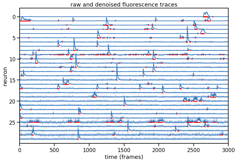
def plot_problem_2(traces, denoised_traces, amplitudes):
    num_neurons, num_frames = traces.shape

    # Plot the traces and our denoised estimates
    scale = torch.quantile(traces, .995, dim=1, keepdims=True)
    offset = -torch.arange(num_neurons)

    # Plot points at the time frames where the (normalized) amplitudes are > 0.05
    sparse_amplitudes = amplitudes / scale
    # sparse_amplitudes = torch.isclose(sparse_amplitudes, 0, atol=0.05)
    sparse_amplitudes[sparse_amplitudes < 0.05] = torch.nan
    sparse_amplitudes[sparse_amplitudes > 0.05] = 0.0

    plt.figure(figsize=(12, 8))
    plt.plot((traces / scale).T + offset , color=palette[0], lw=1, alpha=0.5)
    plt.plot((denoised_traces / scale).T + offset, color=palette[0], lw=2)
    plt.plot((sparse_amplitudes).T + offset, color=palette[1], marker='o', markersize=2)
    plt.xlabel("time (frames)")
    plt.xlim(0, num_frames)
    plt.ylabel("neuron")
    plt.yticks(-torch.arange(0, num_neurons, step=5), 
               labels=torch.arange(0, num_neurons, step=5).numpy())
    plt.ylim(-num_neurons, 2)
    plt.title("raw and denoised fluorescence traces")


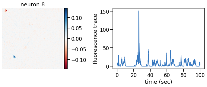
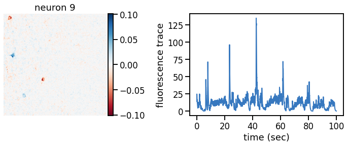
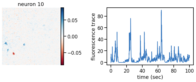
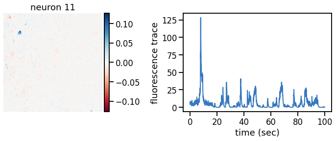
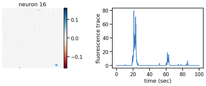
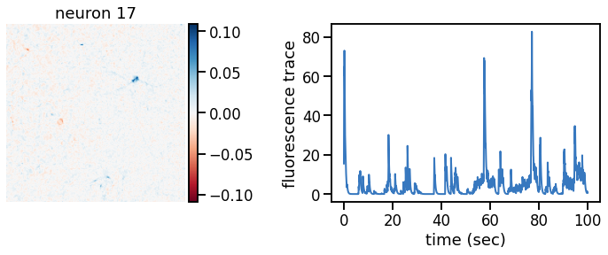
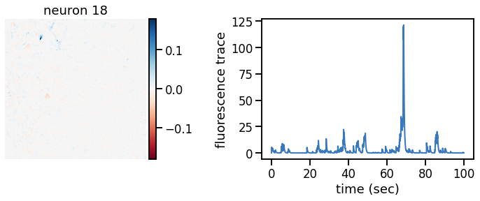
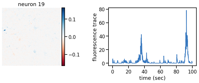
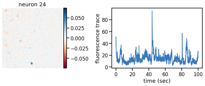
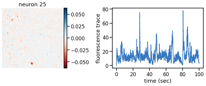
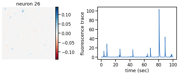
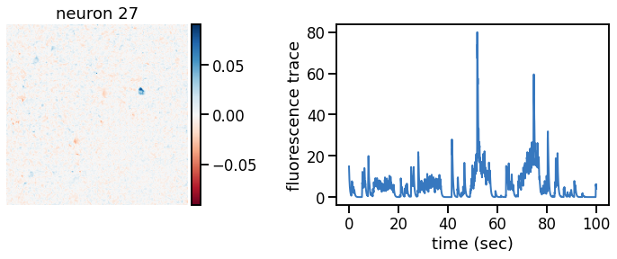
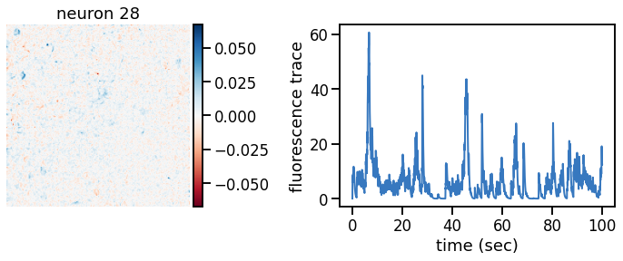
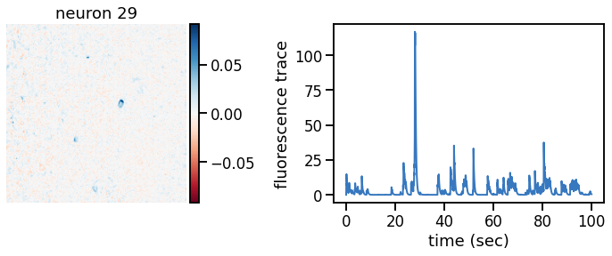
def plot_problem_3(flat_data, params, hypers, plot_bkgd=True, indices=None):
    U = params["footprints"].reshape(-1, height, width)
    u0 = params["bkgd_footprint"].reshape(height, width)
    C = params["traces"]
    c0 = params["bkgd_trace"]
    N, T = C.shape

    if indices is None: 
        indices = torch.arange(N)

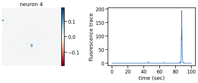
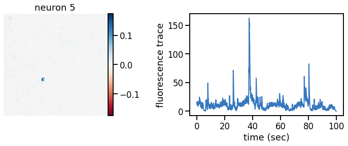
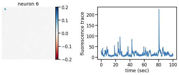
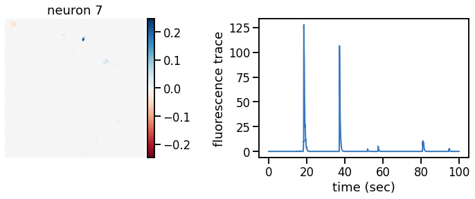
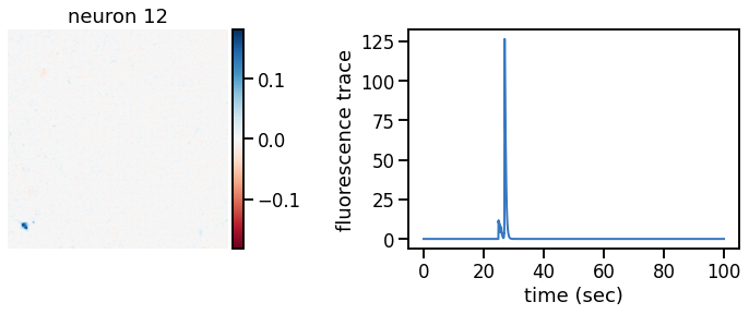
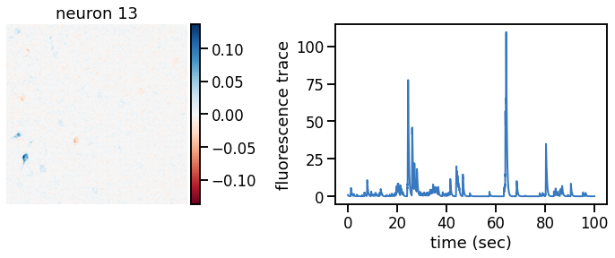
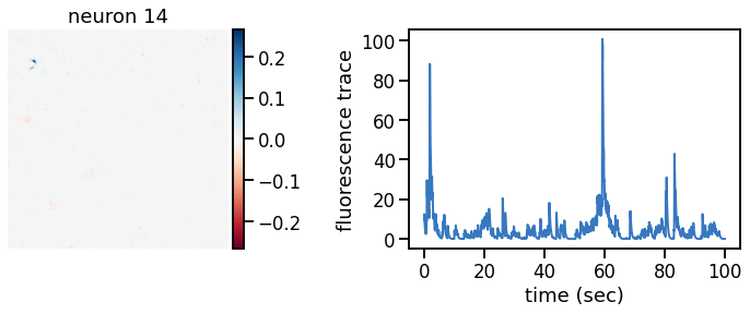
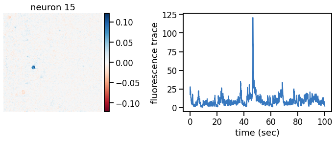
    def _plot_factor(footprint, trace, title):
        fig, ax1 = plt.subplots(1, 1, figsize=(12, 6))
        vlim = abs(footprint).max()
        h = ax1.imshow(footprint, vmin=-vlim, vmax=vlim, cmap="RdBu")
        ax1.set_title(title)
        ax1.set_axis_off()

        # add a colorbar of the same height
        divider = make_axes_locatable(ax1)
        cax = divider.append_axes("right", size="5%", pad="2%")
        plt.colorbar(h, cax=cax)

        ax2 = divider.append_axes("right", size="150%", pad="75%")
        ts = torch.arange(T) / FPS
        ax2.plot(ts, trace, color=palette[0], lw=2)
        ax2.set_xlabel("time (sec)")
        ax2.set_ylabel("fluorescence trace")
        
    if plot_bkgd:
        _plot_factor(u0, c0, "background")

    for k in indices:            
        _plot_factor(U[k], C[k], "neuron {}".format(k))
        

Movie of the data

It takes a minute to render the animation…

# Play the motion corrected movie.
play(data, speedup=5)

Preparing animation. This may take a minute...

Part 1: Initialization

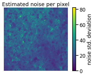
Problem 1a: Estimate the noise at each pixel and standardize

We’ll use a simple heuristic to estimate the noise. With slow calcium responses, most of the high frequency content (e.g. above 8Hz) should be noise. Since Gaussian noise has a flat spectrum (we didn’t prove this but it’s a useful fact to know!), the standard deviation of the high frequency signal should tell us the noise at lower frequencies as well.

In this problem, use butter and sosfilt to high-pass filter the data at 8Hz with a 10-th order Butterworth filter over the time axis (axis=2). Then compute the standard deviation for each pixel using torch.std and the dim keyword argument to get the standard deviation over time for each pixel.

Finally, standardize the data by dividing each pixel by its standard deviation.

# High-pass filter the data at 8Hz using a Butterworth filter.
# That should filter out the calcium transients and give a 
# reasonable estimate of the noise. 

###
# YOUR CODE BELOW
sos = butter(N=..., Wn=..., btype=..., output='sos', fs=...)
noise = sosfilt(...)
noise = torch.tensor(noise, dtype=torch.float32) # convert to tensor
sigmas = torch.std(...)
###
assert sigmas.shape == (height, width)

# Plot the noise standard deviation for each pixel
plt.imshow(sigmas, vmin=0)
plt.axis("off")
plt.title("Estimated noise per pixel")
plt.colorbar(label="noise std. deviation")

# Standardize the data by dividing each frame by the standard deviation
std_data = data / sigmas[:, :, None]

# Check that we got the same answer
assert torch.isclose(sigmas.mean(), torch.tensor(23.4807), atol=1e-4)

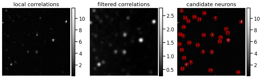
Problem 1b: Find peaks in the local correlation matrix

Step 1 To find candidate neurons, look for places in the image where nearby pixels are highly correlated with one another.

The correlation between pixels \((i,j)\) and \((k,\ell)\) is

\[ \begin{align*} \rho_{ijk\ell} = \frac{1}{T} \sum_{t=1}^T z_{ijt} z_{k\ell t}, \end{align*} \]

where

\[ \begin{align*} z_{ijt} = \frac{x_{ijt} - \bar{x}_{ij}}{\sigma_{ij}} \end{align*} \]

denotes the z-scored data (assume it is zero-padded), \(x_{ijt}\) is the fluorescence at pixel \((ij)\) and frame \(t\), \(\bar{x}_{ij}\) is the average fluorescence at that pixel over time, and \(\sigma_{ij}\) is the standard deviation of fluorescence in that pixel. You’ve already computed the noise level \(\sigma_{ij}\) for each pixel and you computed \(x_{ijt} / \sigma_{ij}\) in Problem 1a. To compute \(z\), simply subtract the mean of the standardized data.

Now define the local correlation at pixel \((i,j)\) to be the average correlation with its neighbors to the north, south, east, and west:

\[ \begin{align*} \bar{\rho}_{ij} = \tfrac{1}{4} \left(\rho_{ij,i+1,j} + \rho_{ij,i-1,j} + \rho_{ij,i,j+1} + \rho_{ij,i,j-1}\right). \end{align*} \]

If \((i,j)\) is a border cell, assume the correlation with out-of-bounds neighbors is zero.

Step 2 Use the gaussian_filter function with a standard deviation sigma=NEURON_WIDTH/4 to smooth the local correlations.

Step 3 Find peaks in the smoothed local correlations using peak_local_max, which we imported from the skimage.feature package. Set a min_distance of 2 and play with the threshold_abs to get 30 neurons, which we think is a reasonable estimate.

# First z-score the data
zscored_data = std_data - std_data.mean(dim=2, keepdims=True)

###
# YOUR CODE BELOW

# Compute the local correlation by summing correlations with 
# neighboring pixels
local_correlations = torch.zeros((height, width))
local_correlations[:, :-1] += torch.mean(...) # W
local_correlations[:,  1:] += torch.mean(...) # E
local_correlations[:-1, :] += torch.mean(...) # S
local_correlations[1:,  :] += torch.mean(...) # N
local_correlations /= 4

# Smooth the local correlations with a Gaussian filter of width 1/4
# the width of a typical neuron. 
filtered_correlations = gaussian_filter(...)
        
# Finally, find peaks in the smoothed local correlations using 
# `peak_local_max`. Set a `min_distance` of 2 and play with the 
# `threshold_abs` to get 30 neurons, which we think is a reasonable estimate.
peaks = peak_local_max(...)

#
###

num_neurons = len(peaks)
print("Found", num_neurons, "candidate neurons")
plot_problem_1d(local_correlations, filtered_correlations, peaks)
assert num_neurons == 30

Found 30 candidate neurons

Problem 1c [Short Answer]: Explain this heuristic

Why are peaks in the local correlations indicative of neurons? Why did you filter the correlations? What would happen if you didn’t use the Gaussian filter, or you used a Gaussian filter of a larger width?

---

Your answer here

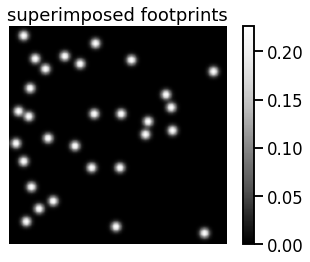
Problem 1d: Initialize the footprints

It’s easer to initialize the footprints in 2D, even though we will eventually ravel the video frames and footprints into vectors. Initialize the 2D footprint to,

\[\begin{split} \begin{align*} u_{k,i,j} \propto \mathcal{N}\left(\begin{bmatrix}i \\ j \end{bmatrix} \,\bigg|\, \begin{bmatrix} \mu_{k,i} \\ \mu_{k,j} \end{bmatrix}, \frac{w}{4} I \right) \end{align*} \end{split}\]

where \(\mu_{k} \in \mathbb{R}^2\) is the location of the peak for neuron \(k\) and \(w\) is the width of a typical neuron. These are the peaks you computed in the previous problem.

There’s a simple trick to initialize the footprints: convolve a Gaussian filter with a matrix that is zeros everywhere except for a one at the location of the peak. The gaussian_filter function with sigma set to NEURON_WIDTH/4 will do this for you.

Finally, normalize the footprints so that \(\|\mathbf{u}_k\|=1\).

footprints = torch.zeros((num_neurons, height, width))

###
# Initialize the footprints as described above
# YOUR CODE BELOW

###

# Check that they're unit norm
assert torch.allclose(torch.linalg.norm(footprints, axis=(1,2)), torch.tensor(1.0))

# Plot the superimpose footprints
plt.imshow(footprints.sum(axis=0), cmap="Greys_r")
plt.axis("off")
plt.title("superimposed footprints")
_ = plt.colorbar()

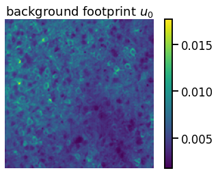
Problem 1e: Initialize the background

Set the spatial background factor \(\mathbf{u}_0\) equal to the median of the standardized data and set the temporal background factor to \(\mathbf{c}_{0} = \mathbf{1}_T\). The median should be more robust to the large spikes than the mean is. Then normalize by dividing \(\mathbf{u}_0\) by its norm \(\|\mathbf{u}_0\|_2\) and multiplying \(\mathbf{c}_0\) by \(\|\mathbf{u}_0\|_2\).

###
# Initialize the background footprint as described above
# YOUR CODE BELOW
bkgd_footprint = ...
bkgd_trace = ...

# Rescale so that spatial background is norm 1
...
###

# Plot the background factor
plt.imshow(bkgd_footprint)
plt.axis("off")
plt.title("background footprint $u_0$")
plt.colorbar()

assert torch.isclose(bkgd_footprint.mean(), torch.tensor(0.0056), atol=1e-4)
assert torch.isclose(bkgd_trace.mean(), torch.tensor(358.4527), atol=1e-4)

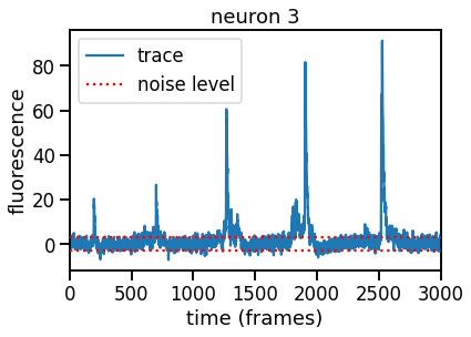
Initialize the traces

We’ll initialize the traces for Part 2 by computing the residual, projecting it onto each footprint in order, and updating the residual by subtracting off each neuron’s contribution.

If we’ve done a good job initializing, the traces should show clear spikes and the noise should be roughly in the range \([-3, +3]\) since the data is standardized to have standard deviation 1.

# This code takes about a minute to run
residual = std_data - torch.einsum('ij,t->ijt', bkgd_footprint, bkgd_trace)
traces = torch.zeros((num_neurons, num_frames))
for k in trange(num_neurons):
    traces[k] = torch.einsum('ij,ijt->t', footprints[k], residual)
    residual -= torch.einsum('ij,t->ijt', footprints[k], traces[k])

# Plot trace for a single neuron
k = 3
plt.plot(traces[k], label="trace")
plt.hlines([-3, 3], 0, num_frames, 
        colors='r', linestyles=':', zorder=10, 
        label="noise level")
plt.legend(loc="upper left")
plt.xlim(0, num_frames)
plt.xlabel("time (frames)")
plt.ylabel("fluorescence")
plt.title("neuron {}".format(k))

# check that we got the same answer using the parameters from parts 1a-1e.
assert torch.isclose(traces[3].mean(), torch.tensor(2.3482))

Part 2: Deconvolving spikes from calcium traces

In this part you’ll use CVXpy to deconvolve the calcium traces by solving a convex optimization problem. CVX is a “Python-embedded modeling language for convex optimization problems,” as the website says. It provides an easy-to-use interface for translating convex optimization problems into code and easy access to a variety of underlying solvers. The key objects are:

• cvx.Variable objects, which specify the variables you wish to optimize with respect to,

• cvx.Minimize objects, which let you specify the objective you wish to minimize,

• cvx.Problem objects, which combine an objective and a set of constraints.

CVX also has lots of helper functions like

• cvx.sum_squares, which computes the sum of squares of an array, and

• cx.norm, which computes norms of the specified order.

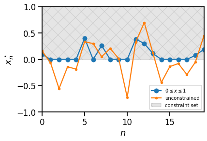
The following example is modified from the CVXpy homepage, linked above. It solves a least-squares problem with box constraints and compares the constrained and unconstrained solutions.

Note: CVXpy is typically used with NumPy arrays, but it can operate on PyTorch tensors too. We’ll just have to remember to conver the results back into tensors in subsequent steps.

# A simple CVX example...

# Problem data.
torch.manual_seed(1)
A = dist.Normal(0.0, 1.0).sample((30, 20))
b = dist.Normal(0.0, 1.0).sample((30,))

# Construct the problem.
x = cvx.Variable(20)
objective = cvx.Minimize(cvx.sum_squares(A @ x - b))
constraints = [0 <= x, x <= 1]
prob = cvx.Problem(objective, constraints)

# The optimal objective value is returned by `prob.solve()`.
# The optimal value for x is stored in `x.value`.
result = prob.solve(verbose=False)

# Plot the constrained optimum vs the unconstrained.
plt.fill_between([0, 19], 0, 1, color='k', alpha=0.1, hatch='x', 
                 label="constraint set")
plt.plot(x.value, '-o', label="$0 \leq x \leq 1$")
plt.plot(torch.linalg.lstsq(A, b, rcond=None)[0], '-', marker='.', 
         label="unconstrained")
plt.xlim(0, 19)
plt.ylim(-1, 1.0)
plt.xlabel("$n$")
plt.ylabel("$x_n^\star$")
plt.legend(loc="lower right", fontsize=10)

<matplotlib.legend.Legend at 0x7ff0baf490d0>

Problem 2a: Solve the convex optimization problem in dual form with CVX

In this part of the lab you’ll use CVXpy to maximize the log joint probability in its dual form:

\[ \begin{align*} \hat{\mathbf{c}}_k, \hat{b}_k = \text{arg min}_{\mathbf{c}_k, b_k} \; \|\mathbf{G} \mathbf{c}_k\|_1 \quad \text{subject to } \quad \|\boldsymbol{\mu}_k - \mathbf{c}_k - b_k\|_2^2 &\leq \theta^2, \; \mathbf{G} \mathbf{c}_k \geq 0, \end{align*} \]

where \(\boldsymbol{\mu}_k = \mathbf{u}_k^\top \mathbf{R} \in \mathbb{R}^T\) is the target for neuron \(k\) and

\[\begin{split} \begin{align*} \mathbf{G} &= \begin{bmatrix} 1 & & & \\ -e^{-1/\tau} & 1 & & \\ 0 & -e^{-1/\tau} & 1 & \\ & 0 & \ddots & \ddots \\ \end{bmatrix} \end{align*} \end{split}\]

is the first order difference matrix. The spike amplitudes (i.e. jumps in the fluorescence) are given by \(\mathbf{a}_k = \mathbf{G} \mathbf{c}_k\), so you can think about the optimization problem as minimizing the \(L^1\) norm of the jumps subject to a non-negativity constraint and an upper bound on the \(L^2\) norm of the difference between the target \(\boldsymbol{\mu}_k\) and the trace \(\mathbf{c}_k\).

Note that this is a slight modification of the problem presented in class:

1. Here we’ve added a bias term \(b_k\), which will be helpful in cases where the target has a nonzero baseline. Accounting for this possibility will lead to more robust estimates of the calcium traces.

2. In class we presented the constraint \(\|\boldsymbol{\mu}_k - \mathbf{c}_k -b\|_2 \leq \theta\). CVXpy does a much better job at solving these “second order cone programs,” so in practice that’s what you should do! For this problem, however, you’ll square both sides, as written in the objective above. Squaring doesn’t change the constraint set, but it will make it easier to compare to the “primal” form you’ll solve in Problem 2d and 2e.

We argued that a reasonable guess for the norm threshold is \(\theta = (1+\epsilon) \sigma \sqrt{T}\). For large \(T\) and good estimates of the target, we should be able to set \(\epsilon\) pretty small. Here, we’ll use a fairly liberal upper bound since we’re working with a short dataset and a poor initial guess.

One of the great things about CVXpy is that it works with SciPy’s sparse matrices. For example, you can use scipy.sparse.diags to construct the \(\mathbf{G}\) matrix. Under the hood, the solver will leverage the sparsity to run in linear time.

def deconvolve(trace, 
               noise_std=1.0, 
               epsilon=1.0,
               tau=GCAMP_TIME_CONST_SEC * FPS,
               full_output=False,
               verbose=False):
    """Deconvolve a noisy calcium trace (aka "target") by solving a 
    the convex optimization problem described above.

    Parameters
    ----------
    trace: a shape (T,) tensor containing the noisy trace.
    noise_std: scalar noise standard deviation $\sigma$
    epsilon: extra slack for the norm constraint. 
        (Typically > 0 and certainly > -1)
    tau: the time constant of the calcium indicator decay.
    full_output: if True, return a dictionary with the deconvolved 
        trace and a bunch of extra info, otherwise just return the trace.
    verbose: flag to pass to the CVX solver to print more info.
    """
    assert trace.ndim == 1
    T = len(trace)

    ###
    # YOUR CODE BELOW

    # Initialize the variable we're optimizing over
    c = cvx.Variable(...)
    b = cvx.Variable(...)

    # Create the sparse matrix G with 1 on the diagonal and 
    # -e^{-1/\tau} on the first lower diagonal
    G = ...

    # set the threshold to (1+\epsilon) \sigma \sqrt{T}
    theta = ...

    # Define the objective function
    objective = cvx.Minimize(...)
    
    # Set the constraints. 
    # PUT THE NORM CONSTRAINT FIRST, THEN THE NON-NEGATIVITY CONSTRAINT!
    constraints = [..., ...]

    # Construct the problem
    prob = cvx.Problem(..., ...)
    ###

    # Solve the optimization problem. 
    try:
        # First try the default solver then revert to SCS if it fails.
        result = prob.solve(verbose=verbose)
    except Exception as e:
        print("Default solver failed with exception:")
        print(e)
        print("Trying 'solver=SCS' instead.")
        # if this still fails we give up!
        result = prob.solve(verbose=verbose, solver="SCS")

    # Make sure the result is finite (i.e. it found a feasible solution)
    if torch.isinf(torch.tensor(result)): 
        raise Exception("solver failed to find a feasible solution!")

    all_results = dict(
        trace=c.value,
        baseline=b.value,
        result=result,
        amplitudes=G @ c.value,
        lagrange_multiplier=constraints[0].dual_value[0]
    )
    assert torch.numel(torch.tensor(constraints[0].dual_value)) == 1, \
        "Make sure your first constraint is on the norm of the residual."

    return all_results if full_output else c.value

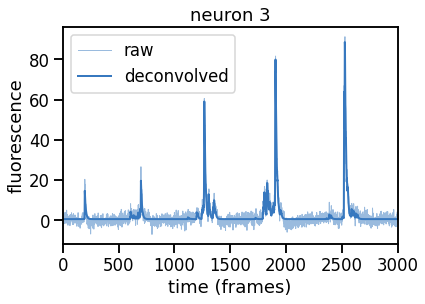
# Solve the deconvolution problem for one neuron
k = 3              # this neuron has particularly high SNR
noise_std = 1.0     # \sigma is 1 since we standardized the data
epsilon = 1.0       # start with a generous tolerance of 2 \sigma \sqrt{T}
dual_results = deconvolve(traces[k], 
                          noise_std=noise_std, 
                          epsilon=epsilon,
                          full_output=True, 
                          verbose=True)

# Plot 
plt.plot(traces[k], color=palette[0], lw=1, alpha=0.5, label="raw")
plt.plot(dual_results["trace"] + dual_results["baseline"], 
         color=palette[0], lw=2, label="deconvolved")
plt.legend(loc="upper left")
plt.xlim(0, num_frames)
plt.xlabel("time (frames)")
plt.ylabel("fluorescence")
_ = plt.title("neuron {}".format(k))

# Check your answer
assert torch.isclose(torch.tensor(dual_results["result"], dtype=torch.float32), 
                     torch.tensor(563.4), 1e-1)

===============================================================================
                                     CVXPY                                     
                                     v1.2.3                                    
===============================================================================
(CVXPY) Jan 25 06:15:47 PM: Your problem has 3001 variables, 2 constraints, and 0 parameters.
(CVXPY) Jan 25 06:15:47 PM: It is compliant with the following grammars: DCP, DQCP
(CVXPY) Jan 25 06:15:47 PM: (If you need to solve this problem multiple times, but with different data, consider using parameters.)
(CVXPY) Jan 25 06:15:47 PM: CVXPY will first compile your problem; then, it will invoke a numerical solver to obtain a solution.
-------------------------------------------------------------------------------
                                  Compilation                                  
-------------------------------------------------------------------------------
(CVXPY) Jan 25 06:15:47 PM: Compiling problem (target solver=ECOS).
(CVXPY) Jan 25 06:15:47 PM: Reduction chain: Dcp2Cone -> CvxAttr2Constr -> ConeMatrixStuffing -> ECOS
(CVXPY) Jan 25 06:15:47 PM: Applying reduction Dcp2Cone
(CVXPY) Jan 25 06:15:47 PM: Applying reduction CvxAttr2Constr
(CVXPY) Jan 25 06:15:47 PM: Applying reduction ConeMatrixStuffing
(CVXPY) Jan 25 06:15:47 PM: Applying reduction ECOS
(CVXPY) Jan 25 06:15:47 PM: Finished problem compilation (took 4.660e-02 seconds).
-------------------------------------------------------------------------------
                                Numerical solver                               
-------------------------------------------------------------------------------
(CVXPY) Jan 25 06:15:47 PM: Invoking solver ECOS  to obtain a solution.
-------------------------------------------------------------------------------
                                    Summary                                    
-------------------------------------------------------------------------------
(CVXPY) Jan 25 06:15:47 PM: Problem status: optimal
(CVXPY) Jan 25 06:15:47 PM: Optimal value: 5.632e+02
(CVXPY) Jan 25 06:15:47 PM: Compilation took 4.660e-02 seconds
(CVXPY) Jan 25 06:15:47 PM: Solver (including time spent in interface) took 2.067e-01 seconds

Plot solutions for a range of \(\epsilon\) (and hence of \(\theta\))

Compute and plot the solutions (in separate figures) for a range of \(\epsilon\) values.

epsilons = [0, 0.25, 0.5, 0.75, 1, 2]
for epsilon in epsilons:
    print("solving with epsilon = ", epsilon)
    
    # deconvolve with this epsilon
    dual_results = deconvolve(traces[k], 
                              noise_std=noise_std, 
                              epsilon=epsilon,
                              full_output=True, 
                              verbose=False)
    
    # Plot 
    plt.figure()
    plt.plot(traces[k], color=palette[0], lw=1, alpha=0.5, label="raw")
    plt.plot(dual_results["trace"] + dual_results["baseline"], 
            color=palette[0], lw=2, label="".format(epsilon))
    plt.legend(loc="upper left", fontsize=10)
    plt.xlim(0, num_frames)
    plt.xlabel("time (frames)")
    plt.ylabel("fluorescence")
    _ = plt.title("neuron {} $\epsilon$ = {:.2f}".format(k, epsilon))

solving with epsilon =  0
solving with epsilon =  0.25
solving with epsilon =  0.5
solving with epsilon =  0.75
solving with epsilon =  1
solving with epsilon =  2

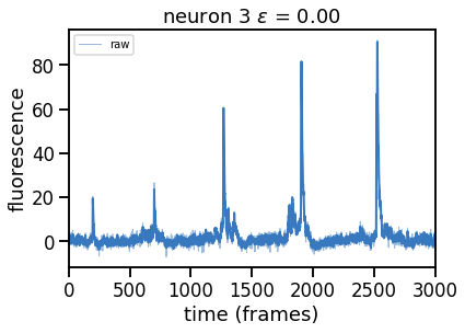
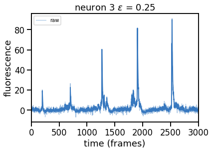
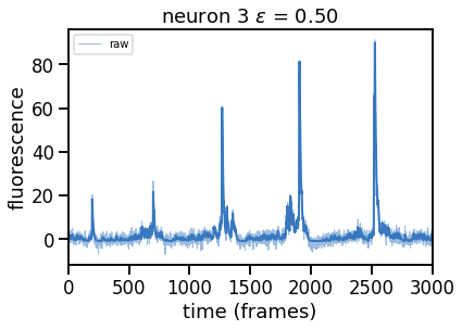
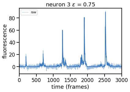
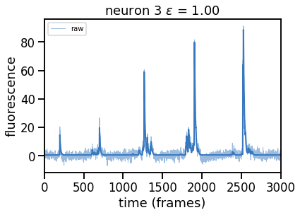
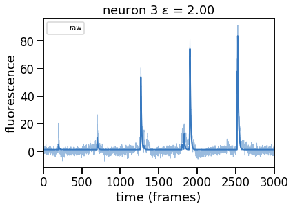
Problem 2b [Short Answer]: Explain these results

How does the solution change as you increase \(\epsilon\) and thereby increase \(\theta\)? Why?

---

Your answer here

Problem 2c [Math]: Relate the dual form to the primal

Replacing the upper bound on the squared norm in Problem 2a with its Lagrangian, we obtain the following “primal” form of the problem:

\[ \begin{align*} \hat{\mathbf{c}}_k, \hat{b}_k = \text{arg min}_{\mathbf{c}_k, b_k} \; \eta (\|\boldsymbol{\mu}_k - \mathbf{c}_k - b_k\|_2^2 - \theta^2) + \|\mathbf{G} \mathbf{c}_k\|_1 \quad \text{subject to } \quad \mathbf{G} \mathbf{c}_k \geq 0, \end{align*} \]

where \(\eta\) is the Lagrange multiplier.

Show that this is equivalent to maximizing the log joint (with a baseline \(b_k\))

\[ \begin{align*} \hat{\mathbf{c}}_k, \hat{b}_k = \text{arg max}_{\mathbf{c}_k, b_k} \mathcal{L}(\mathbf{c}_k, b_k) &= -\frac{1}{2\sigma^2} \|\boldsymbol{\mu}_k - \mathbf{c}_k - b_k\|_2^2 - \lambda_k\|\mathbf{G} \mathbf{c}_k\|_1 \quad \text{subject to } \quad \mathbf{G} \mathbf{c}_k \geq 0 \end{align*} \]

by solving for the value of \(\lambda_k\) (in terms of \(\eta\) and \(\sigma\)) that makes these problems equivalent.

---

Your answer here

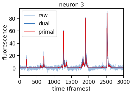
Problem 2d: Solve the problem in primal form with \(\lambda_k\) set to match the dual

Solve the primal problem with CVX using the amplitude rate hyperparameter \(\lambda_k\) that you solved for in Problem 2d and the optimal Lagrange multiplier \(\eta\) output in Problem 2a. In code,

dual_results["lagrange_multiplier"]   # this is \eta

def deconvolve_primal(trace, 
                      amplitude_rate,
                      noise_std=1.0, 
                      tau=GCAMP_TIME_CONST_SEC * FPS,
                      verbose=True,
                      full_output=False):
    """Deconvolve a noisy calcium trace (aka "target") by solving a 
    the convex optimization problem in the primal form.

    Parameters
    ----------
    trace: a shape (T,) tensor containing the noisy trace.
    amplitude_rate: non-negative rate (inverse scale) parameter $\lambda$
    noise_std: scalar noise standard deviation $\sigma$
    tau: the time constant of the calcium indicator decay.
    full_output: if True, return a dictionary with the deconvolved 
        trace and a bunch of extra info, otherwise just return the trace.
    verbose: flag to pass to the CVX solver to print more info.
    """
    assert trace.ndim == 1
    T = len(trace)

    ###
    # YOUR CODE BELOW

    # Initialize the variable we're optimizing over
    c = cvx.Variable(...)
    b = cvx.Variable(...)

    # Create the sparse matrix G with 1 on the diagonal and 
    # -e^{-1/\tau} on the first lower diagonal
    G = ...

    # Define the objective function
    objective = cvx.Minimize(...)
    constraints = [...]
    prob = cvx.Problem(...)
    ###

    # Solve the optimization problem
    result = prob.solve(verbose=verbose)
    if torch.isinf(torch.tensor(result)): 
        raise Exception("solver failed to find a feasible solution!")

    all_results = dict(
        trace=c.value,
        baseline=b.value,
        result=result,
        amplitudes=G @ c.value
    )
    return all_results if full_output else c.value


# Solve the deconvolution problem in the dual form
k = 3               # this neuron has particularly high SNR
noise_std = 1.0     # \sigma is 1 since we standardized the data
epsilon = 1.0       # start with a generous tolerance \epsilon = 1
dual_results = deconvolve(traces[k], 
                          noise_std=noise_std, 
                          epsilon=epsilon,
                          full_output=True, 
                          verbose=True)

###
# Convert the optimal Lagrange multiplier returned in Problem 2a
# to a hyperparameter $\lambda_n$ that sets the rate (inverse scale)
# of the exponential prior on spike amplitudes. The multiplier `eta` is in 
# `dual_results['lagrange_multiplier']` and \sigma is set by `noise_std`.
#
# YOUR CODE BELOW
amplitude_rate = ...
###


# Solve the problem in primal form
primal_results = deconvolve_primal(traces[k], 
                                   amplitude_rate=amplitude_rate, 
                                   verbose=True, 
                                   full_output=True)

# Plot raw, primal, and dual optimal trace for neuron n
plt.plot(traces[k], color=palette[0], lw=1, alpha=0.5, label="raw")
plt.plot(dual_results["trace"] + dual_results["baseline"],
         color=palette[0], ls='-', lw=2, label="dual")
plt.plot(primal_results["trace"] + primal_results["baseline"], 
         color=palette[1], ls='-', lw=1, label="primal")
plt.legend(loc="upper left")
plt.xlim(0, num_frames)
plt.xlabel("time (frames)")
plt.ylabel("fluorescence")
plt.title("neuron {}".format(k))

# Make sure the traces are the same!
primal_diff = abs(dual_results["trace"] - primal_results["trace"]).max()
print("primal and dual solutions match to absolute value: {:.4f}".format(primal_diff))
assert torch.allclose(torch.tensor(dual_results["trace"]), 
                      torch.tensor(primal_results["trace"]), 
                      atol=1e-1)

===============================================================================
                                     CVXPY                                     
                                     v1.2.3                                    
===============================================================================
(CVXPY) Jan 25 06:16:00 PM: Your problem has 3001 variables, 2 constraints, and 0 parameters.
(CVXPY) Jan 25 06:16:00 PM: It is compliant with the following grammars: DCP, DQCP
(CVXPY) Jan 25 06:16:00 PM: (If you need to solve this problem multiple times, but with different data, consider using parameters.)
(CVXPY) Jan 25 06:16:00 PM: CVXPY will first compile your problem; then, it will invoke a numerical solver to obtain a solution.
-------------------------------------------------------------------------------
                                  Compilation                                  
-------------------------------------------------------------------------------
(CVXPY) Jan 25 06:16:00 PM: Compiling problem (target solver=ECOS).
(CVXPY) Jan 25 06:16:00 PM: Reduction chain: Dcp2Cone -> CvxAttr2Constr -> ConeMatrixStuffing -> ECOS
(CVXPY) Jan 25 06:16:00 PM: Applying reduction Dcp2Cone
(CVXPY) Jan 25 06:16:00 PM: Applying reduction CvxAttr2Constr
(CVXPY) Jan 25 06:16:00 PM: Applying reduction ConeMatrixStuffing
(CVXPY) Jan 25 06:16:00 PM: Applying reduction ECOS
(CVXPY) Jan 25 06:16:00 PM: Finished problem compilation (took 3.879e-02 seconds).
-------------------------------------------------------------------------------
                                Numerical solver                               
-------------------------------------------------------------------------------
(CVXPY) Jan 25 06:16:00 PM: Invoking solver ECOS  to obtain a solution.
-------------------------------------------------------------------------------
                                    Summary                                    
-------------------------------------------------------------------------------
(CVXPY) Jan 25 06:16:01 PM: Problem status: optimal
(CVXPY) Jan 25 06:16:01 PM: Optimal value: 5.632e+02
(CVXPY) Jan 25 06:16:01 PM: Compilation took 3.879e-02 seconds
(CVXPY) Jan 25 06:16:01 PM: Solver (including time spent in interface) took 1.985e-01 seconds
===============================================================================
                                     CVXPY                                     
                                     v1.2.3                                    
===============================================================================
(CVXPY) Jan 25 06:16:01 PM: Your problem has 3001 variables, 1 constraints, and 0 parameters.
(CVXPY) Jan 25 06:16:01 PM: It is compliant with the following grammars: DCP, DQCP
(CVXPY) Jan 25 06:16:01 PM: (If you need to solve this problem multiple times, but with different data, consider using parameters.)
(CVXPY) Jan 25 06:16:01 PM: CVXPY will first compile your problem; then, it will invoke a numerical solver to obtain a solution.
-------------------------------------------------------------------------------
                                  Compilation                                  
-------------------------------------------------------------------------------
(CVXPY) Jan 25 06:16:01 PM: Compiling problem (target solver=OSQP).
(CVXPY) Jan 25 06:16:01 PM: Reduction chain: CvxAttr2Constr -> Qp2SymbolicQp -> QpMatrixStuffing -> OSQP
(CVXPY) Jan 25 06:16:01 PM: Applying reduction CvxAttr2Constr
(CVXPY) Jan 25 06:16:01 PM: Applying reduction Qp2SymbolicQp
(CVXPY) Jan 25 06:16:01 PM: Applying reduction QpMatrixStuffing
(CVXPY) Jan 25 06:16:01 PM: Applying reduction OSQP
(CVXPY) Jan 25 06:16:01 PM: Finished problem compilation (took 3.639e-02 seconds).
-------------------------------------------------------------------------------
                                Numerical solver                               
-------------------------------------------------------------------------------
(CVXPY) Jan 25 06:16:01 PM: Invoking solver OSQP  to obtain a solution.
-----------------------------------------------------------------
           OSQP v0.6.2  -  Operator Splitting QP Solver
              (c) Bartolomeo Stellato,  Goran Banjac
        University of Oxford  -  Stanford University 2021
-----------------------------------------------------------------
problem:  variables n = 9001, constraints m = 12000
          nnz(P) + nnz(A) = 35997
settings: linear system solver = qdldl,
          eps_abs = 1.0e-05, eps_rel = 1.0e-05,
          eps_prim_inf = 1.0e-04, eps_dual_inf = 1.0e-04,
          rho = 1.00e-01 (adaptive),
          sigma = 1.00e-06, alpha = 1.60, max_iter = 10000
          check_termination: on (interval 25),
          scaling: on, scaled_termination: off
          warm start: on, polish: on, time_limit: off

iter   objective    pri res    dua res    rho        time
   1  -3.3935e+05   9.13e+01   9.96e+06   1.00e-01   8.41e-03s
 200   1.3940e+04   1.95e-02   9.81e-04   2.69e-02   7.37e-02s
 375   1.3964e+04   2.50e-04   3.24e-05   1.48e-01   1.39e-01s

status:               solved
solution polish:      unsuccessful
number of iterations: 375
optimal objective:    13963.9409
run time:             1.50e-01s
optimal rho estimate: 1.62e-01

-------------------------------------------------------------------------------
                                    Summary                                    
-------------------------------------------------------------------------------
(CVXPY) Jan 25 06:16:01 PM: Problem status: optimal
(CVXPY) Jan 25 06:16:01 PM: Optimal value: 1.396e+04
(CVXPY) Jan 25 06:16:01 PM: Compilation took 3.639e-02 seconds
(CVXPY) Jan 25 06:16:01 PM: Solver (including time spent in interface) took 1.599e-01 seconds
primal and dual solutions match to absolute value: 0.0047

Compute all deconvolved traces and plot them

# Deconvolve each trace and concatenate the results
deconvolved_traces = torch.zeros_like(traces)
amplitudes = torch.zeros_like(traces)
for neuron in trange(num_neurons):
    all_results = deconvolve(traces[neuron], epsilon=0.9, full_output=True)
    deconvolved_traces[neuron] = torch.tensor(all_results["trace"], 
                                              dtype=torch.float32)
    amplitudes[neuron] = torch.tensor(all_results["amplitudes"],
                                      dtype=torch.float32)

plot_problem_2(traces, deconvolved_traces, amplitudes)

Part 3: Demix and deconvolve the calcium imaging video

In this part you’ll write the updates for MAP estimation in the constrained non-negative matrix factorization model.

As in the notes and slides, we will operate on the flattened data and residuals by reshaping the frames into 1d vectors.

Note that unlike CNMF (Pnevmatikakis et al, 2016), we’re not going to constrain the footprints to be non-negative. Instead, we’ll just assume they are normalized, since that’s a bit easier to and it makes a clearer connection to the spike sorting algorithms from the previous lab. It would be a simple extension to enforce non-negativity, and the course notes describe how.

Flatten the pixel dimensions and package the parameters

flat_data = std_data.reshape(-1, num_frames)
flat_footprints = footprints.reshape(num_neurons, -1)
flat_bkgd_footprint = bkgd_footprint.reshape(-1)

# Package the paramters into a dictionary
params = dict(
    traces=torch.zeros((num_neurons, num_frames)),  # C
    bkgd_trace=bkgd_trace,                          # c_0
    footprints=flat_footprints,                     # U
    bkgd_footprint=flat_bkgd_footprint              # u_0
)

# Move the data and params to the GPU
flat_data = flat_data.to(device)
for key in params.keys():
    params[key] = params[key].to(device)

# The hyperparameters specify the number of neurons,
# the noise standard deviation ($\sigma = 1$ since we standardized the data),
# the prior variance of the background trace (something really large),
# and the tolerance for our norm constrain ($\epsilon$).
hypers = dict(
    num_neurons=num_neurons,
    noise_std=1.0,
    bkgd_trace_var=1e6,
    epsilon=1.0,
)

Problem 3a: Write a function to compute the log likelihood given the residual

The log likelihood is

\[\begin{split} \begin{align*} \log p(\mathbf{X} \mid \mathbf{U}, \mathbf{C}) &= \sum_{n=1}^N \sum_{t=1}^T \log \mathcal{N}\left(x_{n,t} \,\bigg|\, \sum_{k=0}^K u_{k,n} c_{k,t}, \sigma^2 \right) \\ \end{align*} \end{split}\]

Write a function to compute the log likelihood given the precomputed residual \(\mathbf{R} = \mathbf{X} - \mathbf{U} \mathbf{C}^\top \).

Hint: Use dist.Normal’s log_prob function.

def log_likelihood_residual(residual, hypers):
    """ Evaluate the log joint probability of the data 
    given the precomputed residual $Y - U^T C - u_0 c_0^T$

    Parameters
    ----------
    residual: a NxT tensor array containing the residual noise
        after subtracting the neuron and background contributions.

    hypers: dictionary of hyperparameters
    """
    ### 
    # YOUR CODE HERE
    lp = ...
    ###
    return lp / residual.numel()
    
# check it on the flat data (as if C and c_0 were zero)
assert torch.isclose(
    log_likelihood_residual(flat_data, hypers), 
    torch.tensor(-4.6855), atol=1e-4)

Problem 3b: Optimize a trace

Optimize a single neuron’s trace using the deconvolve function you wrote in Problem 2a. The target is \(\boldsymbol{\mu}_k = \mathbf{u}_k^\top \mathbf{R}_k\) where \(R_k\) is the residual for this neuron. The residual is given as input to this function.

Note: In your final version, make sure you have verbose=False so that the final code doesn’t print a bunch of unnecessary stuff.

def _update_trace(neuron, residual, params, hypers):
    """Update a single neuron's trace by calling your `deconvolve` function.

    Parameters
    ----------
    neuron: integer index of which neuron to update
    residual: a NxT tensor containing the residual for this neuron.
    params: parameter dictionary
    hypers: hyperparameter dictionary
    """
    footprint = params["footprints"][neuron]
    
    ###
    # YOUR CODE BELOW
    target = ...
    target = target.to("cpu")    # Move to CPU so CVXPy can use it
    trace = deconvolve(...)
    ###

    # Move trace back to device before returning
    trace = torch.tensor(trace, device=device, dtype=torch.float32)
    assert torch.all(torch.isfinite(trace))
    return trace

Problem 3c: Optimize a footprint

Optimize a single neuron’s footprint by setting it to \(\mathbf{u}_k = \frac{\mathbf{R} \mathbf{c}_k}{\|\mathbf{R} \mathbf{c}_k\|}\) where \(\mathbf{R}\) is the given residual and \(\mathbf{c}_k\) is the neuron’s trace.

def _update_footprint(neuron, residual, params, hypers):
    """Update a single neuron's footprint.

    Parameters
    ----------
    neuron: integer index of which neuron to update
    residual: a NxT tensor containing the residual for this neuron.
    params: parameter dictionary
    hypers: hyperparameter dictionary
    """
    trace = params["traces"][neuron]

    ###
    # YOUR CODE BELOW
    footprint = ...
    ###

    assert torch.all(torch.isfinite(footprint))
    assert torch.linalg.norm(footprint).isclose(torch.tensor(1.0))
    return footprint

Problem 3d: Optimize the background

Optimize the background trace by projecting the residual onto the background footprint and shrinking the result slightly,

\[ \begin{align*} \mathbf{c}_0 = \left(\frac{\varsigma_0^2}{\sigma^2 + \varsigma_0^2}\right) \mathbf{u}_0^\top \mathbf{R} \end{align*} \]

where \(\mathbf{R} = \mathbf{X} - \sum_{k=1}^K \mathbf{u}_k\mathbf{c}_k^\top \) is the background residual and \(\varsigma_0^2\) is the prior variance on the background trace. (See the course notes for a derivation.)

Update the background footprint by setting it to,

\[ \begin{align*} \mathbf{u}_0 = \frac{\mathbf{R} \mathbf{c}_0}{\|\mathbf{R} \mathbf{c}_0\|} \end{align*} \]

def _update_bkgd_trace(residual, params, hypers):
    """Update the background trace $c_0$.
    
    Parameters
    ----------
    residual: a NxT tensor containing the residual for the background.
    params: parameter dictionary
    hypers: hyperparameter dictionary
    """
    sigmasq = hypers["noise_std"]**2
    sigmasq_prior = hypers["bkgd_trace_var"]
    footprint = params["bkgd_footprint"]

    ###
    # YOUR CODE BELOW
    shrink_factor = ...
    target = ...
    ###

    # update the latent variables in place
    return shrink_factor * target

def _update_bkgd_footprint(residual, params, hypers):
    """Update the background footprint $u_0$.

    Parameters
    ----------
    residual: a NxT tensor containing the residual for the background.
    params: parameter dictionary
    hypers: hyperparameter dictionary
    """
    bkgd_trace = params["bkgd_trace"]

    ###
    # YOUR CODE BELOW
    bkgd_footprint = ...
    ###
    
    assert torch.all(torch.isfinite(bkgd_footprint))
    assert torch.linalg.norm(bkgd_footprint).isclose(torch.tensor(1.0))
    return bkgd_footprint

Putting it all together

Now we’ll put these steps together into the MAP estimation algorithm. It’s very similar to what you implemented in Lab 2. It amounts to:

• Initialize the residual \(\mathbf{R} = \mathbf{X} - \mathbf{U} \mathbf{C}^\top\)

• Repeat until convergence:

  • For each neuron \(k=1,\ldots,K\):

    • Update the residual to \(\mathbf{R} = \mathbf{R} + \mathbf{u}_k \mathbf{c}_k^\top\)

    • Update the trace \(\mathbf{c}_k\) by applying your deconvolve function from Part 2a to the target \(\boldsymbol{\mu}_k = \mathbf{u}_k^\top \mathbf{R}\)

    • Update the footprint to \(\mathbf{u}_k = \frac{\mathbf{R} \mathbf{c}_k}{\|\mathbf{R} \mathbf{c}_k\|}\)

    • Downdate the residual to \(\mathbf{R} = \mathbf{R} - \mathbf{u}_k \mathbf{c}_k^\top\) using the new footprint and trace

  • Update the background:

    • Update the residual to \(\mathbf{R} = \mathbf{R} + \mathbf{u}_0 \mathbf{c}_0^\top\)

    • Set the background trace to \(\mathbf{c}_0 = \frac{\varsigma_0^2}{\sigma^2 + \varsigma_0^2} \mathbf{u}_0^\top \mathbf{R}\) where \(\varsigma_0^2\) is the prior variance of the background trace. (We will set it to be very large so that we barely shrink the background trace.)

    • Set the background footprint to \(\mathbf{u}_0 = \frac{\mathbf{R} \mathbf{c}_0}{\|\mathbf{R} \mathbf{c}_0\|}\)

    • Downdate the residual to \(\mathbf{R} = \mathbf{R} - \mathbf{u}_0 \mathbf{c}_0^\top\) using the new background footprint and trace.

  • Compute the log likelihood using the residual \(\mathbf{R}\)

def map_estimate(flat_data,
                 params,
                 hypers,
                 num_iters=10,
                 tol=2e-4):
    """Fit the CNMF model via coordinate ascent.
    """
    
    # make a fancy reusable progress bar for the inner loops over neurons.
    outer_pbar = trange(num_iters)
    inner_pbar = trange(hypers["num_neurons"])
    inner_pbar.set_description("updating neurons")

    # initialize the residual
    residual = torch.clone(flat_data)
    residual -= params["footprints"].T @ params["traces"]
    residual -= torch.outer(params["bkgd_footprint"], params["bkgd_trace"])

    # track log likelihoods over iterations
    lls = [log_likelihood_residual(residual, hypers)]
    outer_pbar.set_description("LL: {:.4f}".format(lls[-1]))

    # coordinate ascent
    for itr in outer_pbar:
        
        # update neurons one at a time
        inner_pbar.reset()
        for k in range(hypers["num_neurons"]):
            # update the residual (add $u_k c_k^\top$)
            residual += torch.outer(params["footprints"][k], params["traces"][k])
    
            # update the trace and footprint with the residual
            params["traces"][k] = _update_trace(k, residual, params, hypers)
            params["footprints"][k] = _update_footprint(k, residual, params, hypers)
            
            # downdate the residual (subtract $u_k c_k^\top$)
            residual -= torch.outer(params["footprints"][k], params["traces"][k])

            # step the progress bar
            inner_pbar.update()

        # update the background
        residual += torch.outer(params["bkgd_footprint"], params["bkgd_trace"])
        params["bkgd_trace"] = _update_bkgd_trace(residual, params, hypers)
        params["bkgd_footprint"] = _update_bkgd_footprint(residual, params, hypers)
        residual -= torch.outer(params["bkgd_footprint"], params["bkgd_trace"])
        
        # compute the log likelihood 
        lls.append(log_likelihood_residual(residual, hypers))
        outer_pbar.set_description("LL: {:.4f}".format(lls[-1]))
        
        # check for convergence
        if abs(lls[-1] - lls[-2]) < tol:
            print("Convergence detected!")
            break
    
    return torch.stack(lls), params

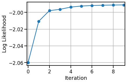
Fit it!

This should take about 2 minutes with a GPU backend.

Note: With the default setting of \(\epsilon\), you will likely see the following warning:

Default solver failed with exception:
Solver 'ECOS' failed. Try another solver, or solve with verbose=True for more information.
Trying 'solver=SCS' instead.
/usr/local/lib/python3.8/dist-packages/cvxpy/problems/problem.py:1337: UserWarning: Solution may be inaccurate. Try another solver, adjusting the solver settings, or solve with verbose=True for more information.

When this happens, the SCS solver can take around 20 seconds to complete. For me, it only happens when updating neuron 28 in the first epoch.

# Fit it!
lls, params = map_estimate(flat_data, params, hypers)

Default solver failed with exception:
Solver 'ECOS' failed. Try another solver, or solve with verbose=True for more information.
Trying 'solver=SCS' instead.

/usr/local/lib/python3.8/dist-packages/cvxpy/problems/problem.py:1337: UserWarning: Solution may be inaccurate. Try another solver, adjusting the solver settings, or solve with verbose=True for more information.
  warnings.warn(

Convergence detected!

# Plot the log likelihoods
plt.plot(lls.to("cpu"), '-o',)
plt.xlabel("Iteration")
plt.xlim(-.1, len(lls) - .9)
plt.ylabel("Log Likelihood")
plt.grid(True)

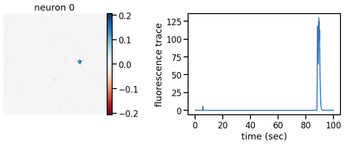
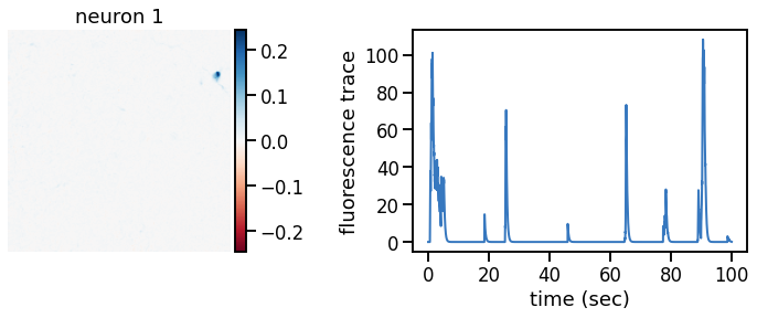
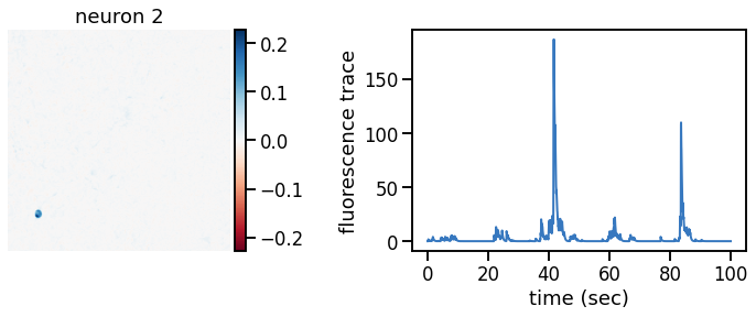
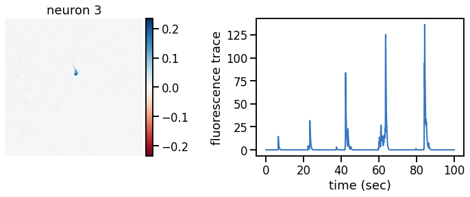
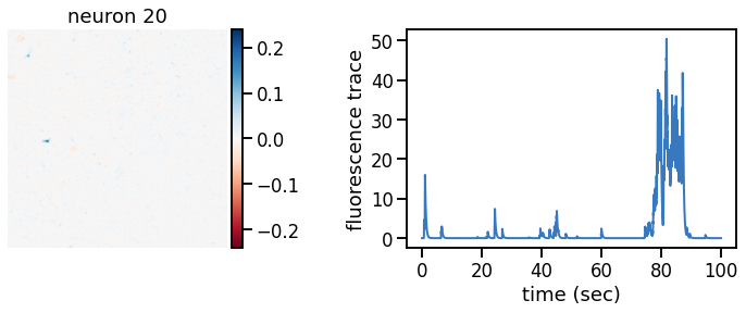
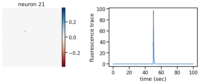
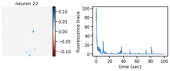
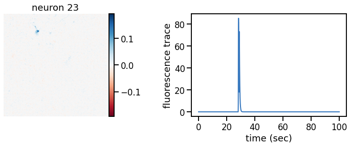
Plot the inferred footprints and traces

# Yes, we know we're creating a lot of figures...
warnings.filterwarnings("ignore")

for key in params.keys():
    params[key] = params[key].to("cpu")
    
plot_problem_3(flat_data, params, hypers)

Make a movie of the data, reconstruction, and residual

Show a movie with the data, reconstruction, and residual side by side. If all goes well, the data should show a nice, clean movie of spiking neurons and the residual should mostly look like white noise. In practice, you’ll probably still see some evidence of neurons in the residual, suggesting that the model still isn’t perfect.

###
# Reconstruct the data and compute the residual.
# Then make a movie of the data, reconstruction, and residual 
# side-by-side.
#
flat_recon = params["footprints"].T @ params["traces"]
flat_recon += torch.outer(params["bkgd_footprint"], params["bkgd_trace"])
flat_residual = flat_data.to("cpu") - flat_recon

# Reshape into image stacks and concatenate along axis=1.
movie = torch.cat([
    flat_data.reshape(height, width, -1).to("cpu"),
    flat_recon.reshape(height, width, -1),
    flat_residual.reshape(height, width, -1),
    ], dim=1)

# Play the movie
play(movie, speedup=5)

Preparing animation. This may take a minute...

Part 4: Discussion

Hopefully you were successful in separating the neurons from the background and noise! Let’s take a minute to reflect on the model and results.

Problem 4a

We mentioned a few times that actual CNMF implementations also constrain the footprints to be non-negative. Without this constraint, you probably found in the plots above (before Problem 3e) that some of these footprints contain negative values. Why is this unrealistic and what are the consequences of omitting this constraint?

---

Your answer here

Problem 4b

You probably noticed that the background has lots of rings in it, like little Cheerios. What could cause that effect?

---

Your answer here

Problem 4c

We assumed that all neurons share the same time constant \(\tau\). Is that reasonable? Without doing any math, describe how you would try to learn per-neuron time constants.

---

Your answer here

Problem 4d

Do you think we can infer the number of underlying action potentials from the amplitude of the jumps in the calcium traces? Why or why not?

---

Your answer here

Author contributions

Please write a short paragraph describing each authors contributions.

---

Your response here

Submission instructions

Formatting: check that your code does not exceed 80 characters in line width. You can set Tools → Settings → Editor → Vertical ruler column to 80 to see when you’ve exceeded the limit.

Download your notebook in .ipynb format and use the following commands to convert it to PDF.

Option 1 (best case): ipynb → pdf Run the following command to convert to a PDF:

jupyter nbconvert --to pdf lab2_teamname.ipynb

Unfortunately, nbconvert sometimes crashes with long notebooks. If that happens, here are a few options:

Option 2 (next best): ipynb → tex → pdf:

jupyter nbconvert --to latex lab2_teamname.ipynb
pdflatex lab2_teamname.tex

Option 3: ipynb → html → pdf:

jupyter nbconvert --to html lab2_teamname.ipynb
# open lab2_teamname.html in browser and print to pdf

Dependencies:

• nbconvert: If you’re using Anaconda for package management,

conda install -c anaconda nbconvert

• pdflatex: It comes with standard TeX distributions like TeXLive, MacTex, etc. Alternatively, you can upload the .tex and supporting files to Overleaf (free with Stanford address) and use it to compile to pdf.

Upload your .ipynb and .pdf files to Gradescope.

Only one submission per team!