Demixing Calcium Imaging Data

Demixing Calcium Imaging Data#

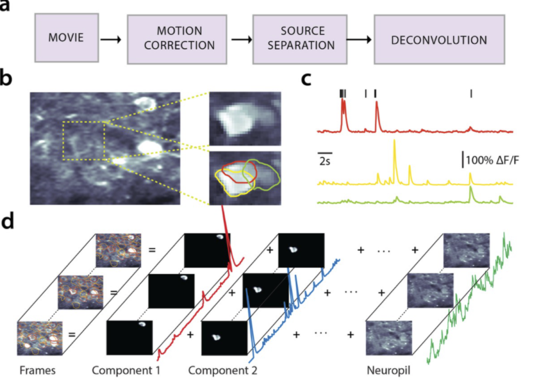
../_images/fig1.png — Fig. 7 a: Pipeline for demixing and deconvolving raw calcium imaging movies. b. An example frame from a 2-photon calcium imaging experiment with three overlapping neurons. c. Demixed calcium fluorescence traces for each of the neurons outlined in b. Spikes above indicate the times of action potentials deconvolved from the red trace. d. Schematic of the model. The (motion corrected) movie frames are modeled as a superposition of fluorescence traces from each component (i.e. neuron) plus background (i.e. neuropil). Each component consists of a spatial factor (i.e. “footprint”) and a temporal factor (i.e. “calcium trace”). This figure was adapted from fig. 1 of Giovannucci *et al.* [2019]#

Electrophysiological (ephys) recordings offer fine timescale measurements of neural spiking, but they have a few key limitations. Even with high density probes like Neuropixels, you only record the cells that happen to be near a recording site. Moreover, ephys methods don’t leverage the wide range of genetic tools available for some model organisms. For example, neuroscientists can control gene expression in specific cell types.

Optical physiology (ophys) techniques leverage these genetic tools to develop an alternative approach to measuring brain activity. The general idea is to alter the DNA of an organism to encode a fluorescent indicator of neuronal activity. These indicators may be targeted to a subset of cells to make them fluoresce when they spike. How can you make fluorescent cells? One way is to alter their DNA so that the neurons of interest produce green fluorescent protein (GFP), which emits bright green light when exposed to blue light; e.g. from a laser. A variety of other fluorescent proteins exist that emit light in other colors, allowing for “multi-spectral” methods that measure activity in multiple color channels. But how can you make cells fluoresce only when they spike? You need to activate the fluorescent protein only when an action potential occurs, and fortunately, there are many ways of accomplishing that feat [Lin and Schnitzer, 2016].

The most mature method of optically measuring neuronal activity is with genetically encoded calcium indicators (GECIs). GECIs bind to calcium ions, which are let into the cell by voltage-gated calcium channels when neurons spike. Once bound, GECIs become fluorescent; for example, GCaMP absorbs blue light and emits green light when bound to calcium. After an action potential, the calcium eventually unbinds and is pumped out of the cell, causing the fluorescence to decay exponentially after spikes. The result is a calcium fluorescence trace with fast peaks followed by exponential decays, as shown in Fig. 7c.

Our goal is to extract the fluorescence traces associated with each neuron in the field of view. The problem is challenging for many reasons. First, the raw video is often corrupted by non-rigid motion artifacts. Second, the neurons may be overlapping, so fluorescence in a single pixel may be attributed to one of many neurons. Third, there is substantial “background” fluorescence coming from out-of-focus tissue (i.e. neuropil). Fourth, the fluorescence is corrupted by noise. On the other hand, we have substantial prior knowledge about fluorescence traces that can guide our inferences. We’ll make use of this prior knowledge in the following model, which is based on the constrained non-negative matrix factorization (CNMF) approach of Vogelstein et al. [2010] and Pnevmatikakis et al. [2016] and implemented in the CaImAn package [Giovannucci et al., 2019]. It is very similar to the methods implemented in Suite2P [Pachitariu et al., 2017].

Constrained Non-negative Matrix Factorization (CNMF)#

Let \(\mathbf{X} \in \mathbb{R}^{N \times T}\) denote a calcium imaging video with \(N\) pixels (assume each frame is flattened into a vector) and \(T\) time frames (typically sampled at around 30 Hz). The entries of this matrix, \(x_{n,t}\), denote the fluorescence intensity measured in pixel \(n\) at time frame \(t\).

Like in the preceding chapter, we assume fluorescence is the sum of intensities from \(K\) neurons, each with its own spatial footprint \(\mathbf{u}_k \in \mathbb{R}^N\) and nonnegative amplitudes \(\mathbf{a}_k \in \mathbb{R}_+^T\). Unlike the previous chapter, however, here we will explicitly model background activity with its own spatial footprint \(\mathbf{u}_0\) and time-varying intensity \(\mathbf{c}_0 \in \mathbb{R}^T\).

The main thing that distinguishes our model for calcium imaging data from our model for spike sorting is that the temporal profile are highly constrained. When the neuron fires an action potential, the calcium concentration (and hence the fluorescence intensity) spikes. As calcium ions unbind from the indicator, the fluorescence decays exponentially. We can model the temporal profile as an exponential function,

\[ \begin{align*} \mathbf{v} &= (1, e^{-1/\tau}, e^{-2/\tau}, \ldots ) \end{align*} \]

where \(\tau \in \mathbb{R}_+\) is the time-constant of intensity decay. The time constant is primarily driven by the calcium indicator (e.g. GCaMP6f vs GCaMP6s), which is usually the same for all neurons. It is easy to generalize the model to allow different time constants for each neuron, if desired.

Since \(\mathbf{v}\) is fixed, calcium imaging models are often formulated in terms of the calcium traces \(\mathbf{c}_k = (c_{k,1}, \ldots, c_{k,T})\), which are the convolution of the spike amplitudes and the temporal profile,

\[ \begin{align*} c_{k,t} = [\mathbf{a}_k \circledast \mathbf{v}]_t = \sum_{d=0}^\infty a_{k-d} e^{-d/\tau}. \end{align*} \]

Putting it all together, the likelihood is,

\[ p(\mathbf{X} \mid \mathbf{U}, \mathbf{C}) = \prod_{n=1}^N \prod_{t=1}^T \mathcal{N}\left(x_{n,t} \,\bigg|\, \sum_{k=1}^K u_{k,n} c_{k,t} + u_{0,n} c_{0,t}, \, \sigma^2 \right). \]

Recursive formulation#

The reason we call this constrained NMF is that the calcium traces are modeled as nonnegative vectors with jumps followed by exponential decays. Thanks to the memoryless property of the exponential function, we can write the model recursively,

\[\begin{split} \begin{align*} c_{k,t} &= \sum_{d=0}^\infty a_{k,t-d} e^{-d/\tau} \\ &= a_{k,t} + \sum_{d=1}^\infty a_{k,t-d} e^{-d/\tau} \\ &= a_{k,t} + \sum_{d=0}^\infty a_{k,t-1-d} e^{-(d+1)/\tau} \\ &= a_{k,t} + e^{-1/\tau} c_{k,t-1}. \end{align*} \end{split}\]

From one frame to the next, the calcium intensity decays by a fraction \(e^{-1/\tau}\), and then a spike of amplitude \(a_{k,t}\) is added.

Back-of-the-envelope calculations with exponentials

Since \(\tau > 0\), \(e^{-1/\tau} < 1\), which captures the fact that calcium traces decay in the absence of spikes. To get a quick estimate of the decay, note that for large \(\tau\), the exponential function is well-approximated by its first ordre Taylor expansion around zero,

\[ e^{-1/\tau} \approx 1-\frac{1}{\tau} \]

For a 300ms time constant and 30Hz frame rate, the time constant (in units of frames) is \(\tau\) = 0.3 sec \(\times\) 30 frames/sec = 9 frames. Thus, between consecutive frames the calcium fluorescence decreases by a fraction of \(1-\frac{1}{9} \approx 0.88\) if there’s no spike.

Prior on intensity traces#

How can we translate our prior on amplitudes into a distribution on calcium traces? Note that \(\mathbf{c}_k\) is an invertible function of the spike amplitudes, \(\mathbf{c}_k = f(\mathbf{a}_k)\). Using the change of measure formula, we can rewrite \(p(\mathbf{c}_k)\) in terms of the prior on amplitudes,

\[ \begin{align*} p(\mathbf{c}_k) &= \left| \tfrac{\mathrm{d} f^{-1}(\mathbf{c}_k)}{\mathrm{d} \mathbf{c}_k} \right| \, p(f^{-1}(\mathbf{c}_k)) \end{align*} \]

In this model, the inverse function is,

\[\begin{split} \begin{align*} \mathbf{a}_k &= f^{-1}(\mathbf{c}_k) = \mathbf{G} \mathbf{c}_k, \quad \text{where} \quad \mathbf{G} = \begin{bmatrix} 1 & & & \\ -e^{-1/\tau} & 1 & & \\ 0 & -e^{-1/\tau} & 1 & \\ & 0 & \ddots & \ddots \\ \end{bmatrix}, \end{align*} \end{split}\]

and its Jacobian is

\[ \begin{align*} \frac{\mathrm{d} f^{-1}(\mathbf{c}_k)}{\mathrm{d} \mathbf{c}_k} &= \mathbf{G}. \end{align*} \]

Since \(G\) is lower triangular, its determinant is simply the product of its diagonal, which in this case is just 1. Intuitively, the determinant of the Jacobian tells us how the volume of a set in \(\mathbb{R}^T\) changes under the linear transformation \(G\). The fact that the determinant of the Jacobian is one tells us that this transformation is volume preserving.

Now we can derive the probability of \(\mathbf{c}_k\) using the change of measure formula,

\[\begin{split} \begin{align*} p(\mathbf{c}_k) &= \left| \tfrac{\mathrm{d} f^{-1}(\mathbf{c}_k)}{\mathrm{d} \mathbf{c}_k} \right| \, p(f^{-1}(\mathbf{c}_k)) \\ &= \left|\mathbf{G} \right| \prod_{t=1}^T \mathrm{Exp}([f^{-1}(\mathbf{c}_k)]_t; \lambda) \\ &= \prod_{t=1}^T \mathrm{Exp}(c_{k,t} - e^{-1/\tau} c_{k,t-1}; \lambda). \end{align*} \end{split}\]

This is just a fancy way of arriving at a very simple observation: the probability of the calcium trace is simply the probability of the corresponding spike amplitudes under the exponential prior.

Completing the model#

For now, let’s assume the spatial footprints are unit-norm, just like in the preceding chapter,

\[ \mathbf{u}_k \sim \mathrm{Unif}(\mathbb{S}_{N-1}) \]

Later, we will discuss a more realistic model in whcih the footprints are constrained to be non-negative.

The other new feature of our model for calcium imaging data is the background model. We will assume the background footprint \(\mathbf{u}_0\) is uniform over \(\mathbb{S}_{N-1}\) as well, but allow the background trace to be positive or negative via a Gaussian prior,

\[ c_{0,t} \sim \mathcal{N}(0, \sigma_0^2). \]

Maximum a posteriori (MAP) estimation#

We’re getting very good at MAP estimation now! The algorithm here will look very similar to that of the last chapter. We will cycle through one neuron at a time, updating its footprint and calcium trace while holding the others fixed. Again, the updates will depend on the residual,

\[ \mathbf{R} = \mathbf{X} - \sum_{j \neq k} \mathbf{u}_j \mathbf{c}_j^\top - \mathbf{u}_0 \mathbf{c}_0^\top \]

where \(\mathbf{R} \in \mathbb{R}^{N \times T}\) has columns \(\mathbf{r}_{t}\) and entries \(r_{n,t}\).

We will add a twist though: we’ll reformulate the update of calcium traces as a convex optimization problem.

Optimizing calcium fluorescence traces#

As a function of the calcium fluorescence for neuron \(k\), the log likelihood is,

\[\begin{split} \begin{align*} \log p(\mathbf{X} \mid \mathbf{U}, \mathbf{C}) &= \sum_{t=1}^T \log \mathcal{N}(\mathbf{r}_{t} \mid \mathbf{u}_{k} c_{k,t}, \, \sigma^2 \mathbf{I}) \\ &= -\frac{1}{2\sigma^2} \sum_{t=1}^T (\mathbf{r}_{t} - \mathbf{u}_{k} c_{k,t})^\top (\mathbf{r}_{t} - \mathbf{u}_{k} c_{k,t}) \\ &= -\frac{1}{2\sigma^2} \sum_{t=1}^T (\mathbf{r}_{t}^\top \mathbf{r}_t - \mathbf{r}_t^\top \mathbf{u}_{k} c_{k,t} + c_{k,t}^2 \mathbf{u}_k^\top \mathbf{u}_{k}) \\ &= -\frac{1}{2\sigma^2} \sum_{t=1}^T (- \mathbf{r}_t^\top \mathbf{u}_{k} c_{k,t} + c_{k,t}^2) + c' \\ \end{align*} \end{split}\]

where we used the fact that \(\mathbf{u}_k^\top \mathbf{u}_k = 1\). We can rewrite this in vector notation,

\[ \begin{align*} \log p(\mathbf{X} \mid \mathbf{U}, \mathbf{C}) &= -\frac{1}{2\sigma^2} ( \mathbf{c}_k^\top \mathbf{c}_k - (\mathbf{R}^\top \mathbf{u}_k)^\top \mathbf{c}_k) + c'. \end{align*} \]

Completing the square, the log likelihood (up to an additive constant) is,

\[ \begin{align*} \log p(\mathbf{X} \mid \mathbf{U}, \mathbf{C}) &= -\frac{1}{2 \sigma^2} \|\mathbf{c}_k - \mathbf{R}^\top \mathbf{u}_k\|_2^2 \end{align*} \]

In other words, it is the squared Euclidean norm of the difference between the calcium trace and the projected residual \(\mathbf{R}^\top \mathbf{u}_k\).

Now consider the log prior as a function of \(\mathbf{c}_k\). It can be expressed as,

\[\begin{split} \begin{align*} \log p(\mathbf{C}) &= \sum_{t=1}^T \log \mathrm{Exp}(c_{k,t} - e^{-1/\tau} c_{k,t-1}; \lambda) \\ &= -\lambda \sum_{t=1}^T (c_{k,t} - e^{-1/\tau} c_{k,t-1}) \\ &= -\lambda \|\mathbf{G} \mathbf{c}_k\|_1 \end{align*} \end{split}\]

Note that everything we have done in this section is exactly analogous to the way we derived the objective for the spike amplitudes in the previous chapter. However, since we’re working with the calcium fluorescence traces — i.e., the convolution of the spike amplitudes and the temporal responses — instead of the spike amplitudes directly, we end up with a slightly different expression. We could, of course, convert back to spike amplitudes and use the same heuristic approach as before. Namely, we could use find_peaks on the cross-correlation of the residual and the exponential decay filter. However, that heuristic required us to set a minimum peak height, \(\lambda \sigma^2\). This formulation suggests an alternative approach.

Dual formulation#

Maximizing the objective above subject to the non-negativity constrain \(\mathbf{c}_k \geq 0\) is equivalent to solving the following optimization problem,

\[ \begin{align*} \mathbf{c}_k^\star = \text{arg} \, \min_{\mathbf{c}_k} \; \|\mathbf{G} \mathbf{c}_k\|_1 \quad \text{subject to } \quad \|\mathbf{c}_k - \mathbf{R}^\top \mathbf{u}_k\|_2 &\leq \theta, \; \mathbf{G} \mathbf{c}_k \geq 0, \end{align*} \]

for some threshold \(\theta\) that depends on \(\lambda\) and \(\sigma^2\).

This is a convex optimization problem. It has a linear objective (\(\|\mathbf{G} \mathbf{c}_k\|_1\)) with linear constraints (\(\mathbf{G} \mathbf{c}_k \geq 0\)) and quadratic constraints (\(\|\mathbf{c}_k - \mathbf{R}^\top \mathbf{u}_k\|_2 \leq \theta\)).

Note

Since \(\mathbf{G}\) is a sparse banded matrix, this optimization problem is tractable even for large \(T\) using standard optimization libraries like CVXpy.

Setting the threshold#

Whereas setting \(\lambda\) was a bit tricky, here we can make a pretty good guess as to what the threshold \(\theta\) should be. Under our model, the vector of differences \(\boldsymbol{\epsilon}_k = (\epsilon_{k,1}, \ldots, \epsilon_{k,T})\) with \(\epsilon_{k,t} = c_{k,t} - \mathbf{r}_t^\top \mathbf{u}_k\) is distributed as,

\[ \boldsymbol{\epsilon}_k \sim \mathcal{N}(0, \sigma^2 \mathbf{I}), \]

or equivalently,

\[ \sigma^{-1} \boldsymbol{\epsilon}_k \sim \mathcal{N}(0, \mathbf{I}). \]

The \(\ell_2\) norm of a vector of \(T\) iid standard normal random variables is itself a random variable, and it follows a chi distribution with \(T\) degrees of freedom,

\[ \|\sigma^{-1} \boldsymbol{\epsilon}_k\|_2 \sim \chi_T. \]

For large \(T\), the chi distribution concentrates around its mode, \(\sqrt{T-1}\), so we expect

\[ \|\mathbf{c}_k - \mathbf{R}^\top \mathbf{u}_k\|_2 \approx \sigma \sqrt{T-1}. \]

A conservative guess for the threshold is \(\theta = (1 + \delta) \sigma \sqrt{T-1}\) with, e.g., \(\delta = \tfrac{1}{4}\).

But how do we estimate the noise variance, \(\sigma^2\)? One option is to fit it as part of our MAP estimation. Another is to note that Gaussian noise has a flat power spectrum. If we high pass filter the data to throw away spikes and other background fluctuations, the result should be white noise, and its variance should be a good estimate of \(\sigma^2\).

The \(\chi\) and \(\chi^2\) distributions

The \(\ell_2\) norm of a vector of iid standard normal random variables \(\mathbf{z} = (z_1, \ldots, z_\nu)\) follows a chi (\(\chi\)) distribution with \(\nu\) degrees of freedom. The sum of squares, \(\mathbf{z}^\top \mathbf{z} = z_1^2 + \ldots z_\nu^2\), follows its sibling, the chi (\(\chi^2\)) squared distribution. The \(\chi^2\) distribution is widely used throughout statistics, with applications to hypothesis testing, the analysis of variance, and as a prior distribution for variances in Bayesian models.

Its density is,

\[ \chi^2(x; \nu) = \frac{1}{2^{\frac{\nu}{2}} \Gamma(\frac{\nu}{2})} x^{\frac{\nu}{2} - 1} e^{-\frac{x}{2}}. \]

Exercise

Show that the \(\chi^2\) distribution is also a special case of the gamma distribution.

Optimizing the background fluorescence#

As a function of the background fluorescence trace \(\mathbf{c}_0\), the log joint probability is,

\[ \begin{align*} \log p(\mathbf{X}, \mathbf{U}, \mathbf{C}) &= -\frac{1}{2\sigma^{2}} \|\mathbf{c}_{0} - \mathbf{R}^\top \mathbf{u}_0\|_2^2 - \frac{1}{2\sigma_0^2} \mathbf{c}_0^\top \mathbf{c}_0 + c', \end{align*} \]

where \(\mathbf{R} = \mathbf{x} - \sum_{k=1}^K \mathbf{u}_k \mathbf{c}_{k}^\top\) denotes the residual.

Both terms in the log probability are quadratic in \(\mathbf{c}_0\). Completing the square yields,

\[ \begin{align*} \log p(\mathbf{X}, \mathbf{U}, \mathbf{C}) = -\frac{1}{2\varsigma_{0}^2} \|\mathbf{c}_0 - \mathbf{c}_0^\star\|_2^2 + c' \end{align*} \]

where

\[\begin{split} \begin{align*} \varsigma_{0}^2 &= \left( \frac{1}{\sigma_0^2} + \frac{1}{\sigma^2} \right)^{-1} = \frac{\sigma^2 \sigma_0^2}{\sigma^2 + \sigma_0^2} \\ \mathbf{c}_0^\star &= \varsigma_{0}^2 \left( \frac{\mathbf{R}^\top \mathbf{u}_0}{\sigma^2} \right) = \frac{\sigma_0^2}{\sigma^2 + \sigma_0^2} (\mathbf{R}^\top \mathbf{u}_0). \end{align*} \end{split}\]

The maximum is attained at \(\mathbf{c}_0^\star\), the residual projected onto the background footprint but shrunk by a factor of \(\sigma_0^2 / (\sigma^2 + \sigma_0^2) < 1\). As the prior variance \(\sigma_0^2\) goes to infinity, the shrinkage factor goes to one and we get simply the projected residual. When the prior variance is small relative to the noise, the estimate is shrunk more toward the prior mean of zero.

Non-negative spatial footprints#

Unlike the spikes observed in voltage recordings, calcium fluorescence should only be positive.\footnote{Strictly speaking, the fluorescence could go below zero if calcium concentrations dip below baseline at some points in time. We’ll disregard these minor effects.} Our model so far allows the spatial footprints \(u_n\) to be positive or negative, as long as they are unit norm. A simple fix is to drop the normalization constraint and instead impose a non-negativity constraint in the form of an exponential prior on the footprints,

\[ \begin{align*} p(\{\mathbf{u}_k\}_{k=1}^K) = \prod_{k=1}^K \prod_{n=1}^N \mathrm{Exp}(u_{k,n} \mid \lambda_u), \end{align*} \]

where \(\lambda_u\) is the rate (i.e. inverse scale) hyperparameter. Likewise, we place an exponential prior on the background footprint,

\[ \begin{align*} p(\mathbf{u}_0) &= \prod_{n=1}^N \mathrm{Exp}(u_{0,n} \mid \lambda_{u_0}). \end{align*} \]

Since the background footprint will typically not be sparse, we set \(\lambda_{u_0} \ll \lambda_u\), which increases the prior mean and corresponds to weaker regularization of the background footprint.

Under this model, the log joint probability as a function of \(u_{k,n}\) is,

\[\begin{split} \begin{align*} \log p(\mathbf{X}, \mathbf{U}, \mathbf{C}) &= -\frac{1}{2 \sigma^2} \sum_{t=1}^T \|r_{n,t} - u_{k,n} c_{k,t}\|_2^2 - \lambda_{u} u_{k,n} + c' \\ &= -\frac{1}{2 \sigma^2} (\mathbf{r}_n - u_{k,n} \mathbf{c}_{k})^\top (\mathbf{r}_n - u_{k,n} \mathbf{c}_{k}) - \lambda_{u} u_{k,n} + c' \\ &= -\frac{\alpha}{2} u_{k,n}^2 + \beta u_{k,n} + c'' \end{align*} \end{split}\]

where \(\mathbf{r}_n\) is the \(n\)-th row of \(\mathbf{R}\) and,

\[\begin{split} \begin{align*} \alpha &= \frac{\mathbf{c}_k^\top \mathbf{c}_k}{\sigma^2} \\ \beta &= \frac{\mathbf{r}_n^\top \mathbf{c}_k}{\sigma^2} - \lambda_u \end{align*} \end{split}\]

The maximum, subject to \(u_{k,n} \geq 0\), is at \(\max\{0, \beta/\alpha\}\), or,

\[ \begin{align*} u_{k,n} = \max \left\{0, \frac{\mathbf{c}_k^\top \mathbf{r}_{n} - \sigma^2 \lambda_u}{\mathbf{c}_k^\top \mathbf{c}_k} \right\} \end{align*} \]

The same steps lead to

\[ \begin{align*} u_{0,n} = \max \left\{0, \frac{\mathbf{c}_0^\top \mathbf{r}_{n} - \sigma^2 \lambda_{u_0}}{\mathbf{c}_0^\top \mathbf{c}_0} \right\} \end{align*} \]

for the background footprint.

Again, the hyperparameters \(\lambda_u\) and \(\lambda_{u_0}\) are a bit of a nuisance. It’s not obvious how to set the a priori. We can expect the spatial footprints to be spatially localized, but that leads to dependencies between pixels that are challenging to optimize. One simpler heuristic is to tune \(\lambda_u\) so that the number of nonzero pixels in the footprint is about the size of an average neuron.

Alternative approach#

Another way is to solve for the all weights associated with a single pixel. This approach is attractive because the problem factors over pixels.

As a function of the weights associated with pixel \(n\), the log probability is,

\[\begin{split} \begin{align*} &\log p(\mathbf{X}, \mathbf{U}, \mathbf{C}) \\ &\qquad -\frac{1}{2\sigma^2} \sum_{t=1}^T \left(x_{n,t} - \sum_{k=1}^K u_{k,n} c_{k,t} - u_{0,n} c_{0,t} \right)^2 - \lambda_u \sum_{k=1}^K u_{k,n} - \lambda_{u_0} u_{0,n}. \end{align*} \end{split}\]

To put this in a more natural form, let \(\tilde{u}_{0,n} = \tfrac{\lambda_{u_0}}{\lambda_u} u_{0,n}\) and \(\tilde{\mathbf{u}}_n = (\tilde{u}_{0,n}, u_{1,n}, \ldots, u_{K,n})^\top\). Likewise, let \(\tilde{c}_{0,t} = \tfrac{\lambda_{u}}{\lambda_{u_0}} c_{0,t}\), \(\tilde{\mathbf{c}}_0 = (\tilde{c}_{0,1}, \ldots, \tilde{c}_{0,T})^\top\), and,

\[\begin{split} \begin{align*} \tilde{C} &= \begin{bmatrix} | & | & & | \\ \tilde{\mathbf{c}}_0 & \mathbf{c}_1 & \cdots & \mathbf{c}_K \\ | & | & & | \end{bmatrix}. \end{align*} \end{split}\]

Then,

\[\begin{align*} \log p(\mathbf{X}, \mathbf{U}, \mathbf{C}) &= -\frac{1}{2\sigma^2} \|\mathbf{x}_{n} - \tilde{\mathbf{C}} \tilde{\mathbf{u}}_{n} \|_2^2 -\lambda_u \| \tilde{\mathbf{u}}_{n}\|_1, \end{align*} \]

where \(\mathbf{x}_n\) is the \(n\)-th row of \(\mathbf{X}\) and

This is a convex optimization problem just like one above for the fluorescence traces. Like above, we can solve its dual problem with a constraint,

\[ \begin{align*} \tilde{\mathbf{u}}_n^\star = \text{arg} \, \min_{\tilde{\mathbf{u}}_n} \; \|\tilde{\mathbf{u}}_n\|_1 \quad \text{s.t.} \quad \|\mathbf{x}_{n} - \tilde{\mathbf{C}} \tilde{\mathbf{u}}_{n}\|_2 &\leq (1 + \delta) \sigma \sqrt{T-1}, \; \tilde{\mathbf{u}}_n \geq 0, \end{align*} \]

A simpler way is to note that this is a standard \(\ell_1\)-regularized linear regression problem, and it can be solved with a variety of methods including the LARS algorithm, even when the weights are constrained to be non-negative.

Better background models#

The fluorescence measured at the camera does not arise solely from cells in imaging plane, but also from photons emitted by out-of-focus tissue. This is particularly evident in widefield microscopy and one-photon microendoscopy where the entire sample is illuminated by a light source and the measured fluorescence comes from neurons throughout the sample. Other microscopy methods like confocal and two-photon microscopy reduce out-of-focus light, but the measured fluorescence always has some contribution from tissue outside the imaging plane. The result is a blurry, time-varying background signal that adds to the light collected from the in-focus cells.

So far, we’ve modeled the “background” fluorescence with a rank one model, \(\mathbf{u}_0 \mathbf{c}_0^\top\). This isn’t a bad approximation, but it doesn’t account for background intensities that fluctuate separately in different parts of the video frame. There have been a few suggestions for how to address this limitation. One is to simply increase the rank of the background model, however, without constraints there’s nothing to prevent the background model from also capturing neural signals of interest.

A natural constraint on the background is that it is spatially smoooth, at least on the length-scales of single neurons. There are many ways to incorporate such a constraint; a simple and straightforward way is with basis functions. Let, \(B \in \mathbb{N}\) denote the number of background basis functions, and let \(\boldsymbol{\phi}_b \in \mathbb{R}_+^{N}\) denote a fixed, non-negative basis function over the pixels. For example, we could set,

\[\begin{split} \begin{align*} \boldsymbol{\phi}_{b,n} &\propto \mathcal{N} \left( \begin{bmatrix} x_n \\ y_n \end{bmatrix} \, \bigg| \, \begin{bmatrix} \mu_{x,b} \\ \mu_{y,b} \end{bmatrix}, \eta^2 I \right), \end{align*} \end{split}\]

where \((x_n, y_n)\) denotes the location of pixel \(n\) in xy-coordinates of the image, \((\mu_{x,b}, \mu_{y,b})\) denote the center of the \(b\)-th basis function in xy-coordinates of the image, and \(\eta\) denotes the width of the basis function in pixels. These are called radial basis functions. We typically set their width to be 5-6 times larger than the size of a neuron and tile them so they cover the image. As above, we normalize the basis functions so that \(\|\boldsymbol{\phi}_b\|_2 = 1\).

Then we model the fluorescence as a sum of neuron factors plus the a weighted combination of the basis functions, which capture background variation,

\[ \begin{align*} \mathbf{x}_t &\sim \mathcal{N} \left( \sum_{k=1}^K \mathbf{u}_k c_{k,t} + \sum_{b=1}^B \boldsymbol{\phi}_{b} f_{b,t}, \, \sigma^2 \mathbf{I} \right), \end{align*} \]

where \(f_{b,t}\) is background fluorescence for basis function \(b\) at time \(t\).

Conclusion#

Calcium imaging, and optical physiology more generally, offers a powerful and complementary toolkit for measuring neural activity in genetically defined cell types.

Methods for demixing and deconvolving calcium fluorescence traces are similar to those for spike sorting — again, convolutional matrix factorization was the key idea.

With calcium traces, though, we can place more stringent constraints on the form of the temporal response. It’s well-approximated as an exponential decay. This allows us to frame the problem in a new way that leverages convex optimization techniques.