Lab 4: Generalized Linear Models

STATS320: Machine Learning Methods for Neural Data Analysis

Stanford University. Winter, 2023.

---

Team Name: Your team name here

Team Members: Names of everyone on your team here

Due: 11:59pm Thursday, Feb 16, 2023 via GradeScope

---

In this lab, you’ll build generalized linear models (GLMs) and convolutional neural network (CNN) models of retinal ganglion cell (RGC) responses to visual stimuli. You’ll use PyTorch to implement the models and fit them to a dataset kindly provided by the Baccus Lab (Stanford University), which they studied in the “Deep Retina” paper (McIntosh et al, 2016).

References:

McIntosh, Lane T., Niru Maheswaranathan, Aran Nayebi, Surya Ganguli, and Stephen A. Baccus. “Deep Learning Models of the Retinal Response to Natural Scenes.” Advances in Neural Information Processing (NeurIPS), 2017.

Setup

import torch
import torch.nn as nn
import torch.nn.functional as F
from torch.utils.data import Dataset, DataLoader
import torch.optim as optim
from torch.optim import lr_scheduler
from torch.distributions import Poisson


import h5py
import matplotlib.pyplot as plt
import seaborn as sns
from tqdm.auto import trange
from copy import deepcopy


# Specify that we want our tensors on the GPU and in float32
device = torch.device('cuda')
dtype = torch.float32

Helper functions for plotting

Show code cell content Hide code cell content

#@title
sns.set_context("notebook")

# initialize a color palette for plotting
palette = sns.xkcd_palette(["windows blue",
                            "red",
                            "medium green",
                            "dusty purple",
                            "orange",
                            "amber",
                            "clay",
                            "pink",
                            "greyish"])

def plot_stimulus_weights(glm):
    num_neurons = glm.num_neurons
    max_delay = glm.max_delay

    fig, axs = plt.subplots(num_neurons, 3, figsize=(8, 4 * num_neurons), 
                            gridspec_kw=dict(width_ratios=[1, 1.9, .1]))

    temporal_weights = glm.temporal_conv.weight[:, 0].to("cpu").detach()
    bias = glm.temporal_conv.bias.to("cpu").detach()
    spatial_weights = glm.spatial_conv.weight.to("cpu").detach()
    spatial_weights = spatial_weights.reshape(num_neurons, 50, 50)

    # normalize and flip the spatial weights
    for n in range(num_neurons):
        # Flip if spatial weight peak is negative
        if torch.allclose(spatial_weights[n].min(), 
                       -abs(spatial_weights[n]).max()):
            spatial_weights[n] = -spatial_weights[n]
            temporal_weights[n] = -temporal_weights[n]

        # Normalize
        scale = torch.linalg.norm(spatial_weights[n])
        spatial_weights[n] /= scale
        temporal_weights[n] *= scale

    # Set the same limits for each neuron
    vlim = abs(spatial_weights).max()
    ylim = abs(temporal_weights).max()
    
    for n in range(num_neurons):
        axs[n, 0].plot(torch.arange(-max_delay+1, 1) * 10, temporal_weights[n])
        axs[n, 0].set_ylim(-ylim, ylim)
        axs[n, 0].plot(torch.arange(-max_delay+1, 1) * 10, torch.zeros(max_delay), ':k')
        if n < num_neurons - 1:
            axs[n, 0].set_xticklabels([])
        else:
            axs[n, 0].set_xlabel("$\Delta t$ [ms]")

        im = axs[n, 1].imshow(spatial_weights[n], 
                              vmin=-vlim, vmax=vlim, cmap="RdBu")
        axs[n, 1].set_axis_off()
        axs[n, 1].set_title("neuron {}".format(n + 1))
        plt.colorbar(im, cax=axs[n, 2])


def plot_coupling_weights(glm):
    # Get the weights and flip them to get time after spike
    W = glm.coupling_conv.weight.to("cpu").detach()
    # W = W[:, :, ::-1]
    W = torch.flip(W, dims=(2,))
    num_neurons = W.shape[0]
    wlim = abs(W).max()
    dt = 10 * torch.arange(W.shape[2])

    fig, axs = plt.subplots(num_neurons, num_neurons, figsize=(12, 12), 
                            sharex=True, sharey=True)
    for i in range(num_neurons):
        for j in range(num_neurons):
            axs[i, j].plot(dt, 0 * dt, ':k')
            axs[i, j].plot(dt, W[i, j])
            axs[i, j].set_ylim(-wlim, wlim)
            axs[i, j].set_title("${} \\to {}$".format(j, i))

            if i == num_neurons - 1:
                axs[i, j].set_xlabel("$\Delta t$ [ms]")
    plt.tight_layout()

def plot_cnn_subunits_1(cnn):
    num_subunits = cnn.num_subunits_1
    max_delay = cnn.max_delay

    fig, axs = plt.subplots(num_subunits, 3, figsize=(8, 4 * num_subunits), 
                            gridspec_kw=dict(width_ratios=[1, 1.9, .1]))

    temporal_weights = cnn.temporal_conv.weight[:, 0].to("cpu").detach()
    bias = cnn.temporal_conv.bias.to("cpu").detach()
    spatial_weights = cnn.spatial_conv.weight.to("cpu").detach()
    spatial_weights = spatial_weights[:, 0, :, :]

    # normalize and flip the spatial weights
    for n in range(num_subunits):
        # Flip if spatial weight peak is negative
        if torch.allclose(spatial_weights[n].min(), 
                    -abs(spatial_weights[n]).max()):
            spatial_weights[n] = -spatial_weights[n]
            temporal_weights[n] = -temporal_weights[n]

        # Normalize
        scale = torch.linalg.norm(spatial_weights[n])
        spatial_weights[n] /= scale
        temporal_weights[n] *= scale

    # Set the same limits for each neuron
    vlim = abs(spatial_weights).max()
    ylim = abs(temporal_weights).max()
    
    for n in range(num_subunits):
        axs[n, 0].plot(torch.arange(-max_delay+1, 1) * 10, temporal_weights[n])
        axs[n, 0].set_ylim(-ylim, ylim)
        axs[n, 0].plot(torch.arange(-max_delay+1, 1) * 10, torch.zeros(max_delay), ':k')
        if n < num_subunits - 1:
            axs[n, 0].set_xticklabels([])
        else:
            axs[n, 0].set_xlabel("$\Delta t$ [ms]")

        im = axs[n, 1].imshow(spatial_weights[n], 
                              vmin=-vlim, vmax=vlim, cmap="RdBu")
        axs[n, 1].set_axis_off()
        axs[n, 1].set_title("subunit 1,{}".format(n + 1))
        plt.colorbar(im, cax=axs[n, 2])

def plot_cnn_subunits2(cnn):
    cnn_filters_2 = cnn.layer2.weight.to("cpu").detach()

    fig, axs = plt.subplots(cnn.num_subunits_2, 
                            cnn.num_subunits_1,
                            figsize=(4 * cnn.num_subunits_2,
                                    4 * cnn.num_subunits_1),
                            sharex=True, sharey=True)
    vlim = abs(cnn_filters_2).max()
    for i in range(cnn.num_subunits_2):
        for j in range(cnn.num_subunits_1):
            axs[i, j].imshow(cnn_filters_2[i, j], 
                            vmin=-vlim, vmax=vlim, cmap="RdBu")
            
            axs[i, j].set_title('subunit 1,{} $\\to$ 2,{}'.format(j+1,i+1))
            

Helper function to train a Pytorch model.

We’ve slightly modified the train_model function from the previous lab. This version keeps track of the model with the best validation loss over the course of the training epochs.

Show code cell content Hide code cell content

#@title 
def train_model(model, 
                train_dataset, 
                val_dataset,
                objective,
                regularizer=None,
                num_epochs=100, 
                lr=0.1,
                momentum=0.9,
                lr_step_size=25,
                lr_gamma=0.9):
    # progress bars
    pbar = trange(num_epochs)
    pbar.set_description("---")
    inner_pbar = trange(len(train_dataset))
    inner_pbar.set_description("Batch")

    # data loaders for train and validation
    train_dataloader = DataLoader(train_dataset, batch_size=1)
    val_dataloader = DataLoader(val_dataset, batch_size=1)
    dataloaders = dict(train=train_dataloader, val=val_dataloader)

    # use standard SGD with a decaying learning rate
    optimizer = optim.SGD(model.parameters(), 
                          lr=lr, 
                          momentum=momentum)
    scheduler = lr_scheduler.StepLR(optimizer, 
                                    step_size=lr_step_size, 
                                    gamma=lr_gamma)
    
    # Keep track of the best model
    best_model_wts = deepcopy(model.state_dict())
    best_loss = 1e8

    # Track the train and validation loss
    train_losses = []
    val_losses = []
    for epoch in range(num_epochs):
        for phase in ['train', 'val']:
            # set model to train/validation as appropriate
            if phase == 'train':
                model.train()
                inner_pbar.reset()
            else:
                model.eval()
            
            # track the running loss over batches
            running_loss = 0
            running_size = 0
            for datapoint in dataloaders[phase]:
                stim_t = datapoint['stimulus'].squeeze(0)
                spikes_t = datapoint['spikes'].squeeze(0)
                if phase == "train":
                    with torch.set_grad_enabled(True):
                        optimizer.zero_grad()
                        # compute the model output and loss
                        output_t = model(stim_t, spikes_t)
                        loss_t = objective(output_t, spikes_t)
                        # only add the regularizer in the training phase
                        if regularizer is not None:
                            loss_t += regularizer(model)

                        # take the gradient and perform an sgd step
                        loss_t.backward()
                        optimizer.step()
                    inner_pbar.update(1)
                else:
                    # just compute the loss in validation
                    output_t = model(stim_t, spikes_t)
                    loss_t = objective(output_t, spikes_t)

                assert torch.isfinite(loss_t)
                running_loss += loss_t.item()
                running_size += 1
            
            # compute the train/validation loss and update the best
            # model parameters if this is the lowest validation loss yet
            running_loss /= running_size
            if phase == "train":
                train_losses.append(running_loss)
            else:
                val_losses.append(running_loss)
                if running_loss < best_loss:
                    best_loss = running_loss
                    best_model_wts = deepcopy(model.state_dict())

        # Update the learning rate
        scheduler.step()

        # Update the progress bar
        pbar.set_description("Epoch {:03} Train {:.4f} Val {:.4f}"\
                             .format(epoch, train_losses[-1], val_losses[-1]))
        pbar.update(1)

    # load best model weights
    model.load_state_dict(best_model_wts)

    return torch.tensor(train_losses), torch.tensor(val_losses)

Load the data

Load the data from the HDF5 file.

• Each file contains a train and test group.

• Each group contains:

  • time: length frames array of timestamps

  • stimulus: a frames x 50 x 50 video taken at ~100Hz

  • response: a group with

    • binned: cells x frames array of spike counts (for the training data) or rates (for the test data) in each bin

    • firing_rate_xms where x is 5, 10, or 20 milliseconds

!wget -nc https://www.dropbox.com/s/gmgus2rm4sks6b8/whitenoise.h5
# !wget -nc https://www.dropbox.com/s/gj8jf50v7dzy4ew/naturalscene.h5

File ‘whitenoise.h5’ already there; not retrieving.

# Load the white noise data
f = h5py.File("whitenoise.h5", mode='r')
frame_rate = 100
times = torch.tensor(f['train']['time'][:], dtype=dtype)
stimulus = torch.tensor(f['train']['stimulus'][:], dtype=torch.uint8)
spikes = torch.tensor(f['train']['response']['binned'][:].T, dtype=dtype)
test_times = torch.tensor(f['test']['time'][:], dtype=dtype)
test_stimulus = torch.tensor(f['test']['stimulus'][:], dtype=torch.uint8)
test_rates = torch.tensor(f['test']['response']['binned'][:, :-1].T, dtype=dtype)

# Get the size of the training data
num_frames, height, width = stimulus.shape
_, num_neurons = spikes.shape

Part 1: Plot the data

Always visualize your data first!

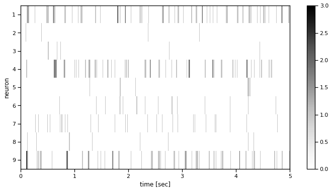
Problem 1a: Plot a slice of the spike train

Write a function to imshow a slice of the data. Add a colorbar and label your axes!

# Plot a few seconds of the spike train
def plot_spike_train(spikes, t_start, t_stop, figsize=(12, 6)):
    """
    `imshow` a window of the spike count matrix.

    spikes:  time x neuron spike count matrix
    t_start: time (in seconds) of the start of the window
    t_stop:  time (in seconds) of the end of the window
    figsize: width and height of the figure in inches
    """
    plt.figure(figsize=figsize)

    ###
    # YOUR CODE BELOW
    
    ###

plot_spike_train(spikes, 0, 5)

Problem 1b: Compute the baseline firing rate for each neuron

Print the mean firing rate for each neuron (on the training data) in spikes per second.

###
# YOUR CODE BELOW
print("Mean firing rates:")
for n in range(num_neurons):
    print("  neuron {}: {:.4f} spk/sec".format(...))
#
###

Mean firing rates:
  neuron 1: 7.1598 spk/sec
  neuron 2: 1.9219 spk/sec
  neuron 3: 1.9822 spk/sec
  neuron 4: 6.2960 spk/sec
  neuron 5: 1.4038 spk/sec
  neuron 6: 1.3310 spk/sec
  neuron 7: 1.8496 spk/sec
  neuron 8: 0.4672 spk/sec
  neuron 9: 3.7988 spk/sec

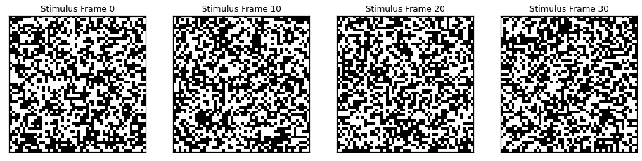
Plot a few frames of the stimulus

Plot the 0th, 10th, 20th, and 30th frames of stimulus in grayscale.

# Plot a few frames of stimulus
def plot_stimulus(stimulus, frame_inds, n_cols=4, panel_size=4):
    num_frames = len(frame_inds)
    n_rows = int(torch.ceil(torch.tensor(num_frames / n_cols)))
    fig, axs = plt.subplots(
        n_rows, n_cols, figsize=(n_cols * panel_size, n_rows * panel_size))
    for ax, ind in zip(axs.ravel(), frame_inds):
        ax.imshow(stimulus[ind], cmap="Greys")
        ax.set_title("Stimulus Frame {}".format(ind))
        ax.set_xticks([])
        ax.set_yticks([])
    for ax in axs.ravel()[len(frame_inds):]:
        ax.set_visible(False)
    
plot_stimulus(stimulus, [0, 10, 20, 30])

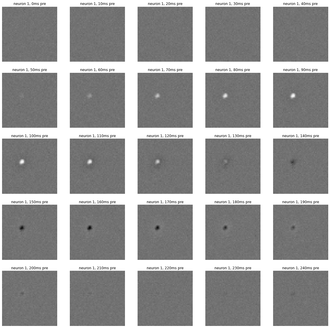
Problem 1c: Compute and plot the spike triggered average

The spike triggered average for neuron \(n\) is the average stimulus in the lead-up to a spike by that neuron.

Formally, let \(A_n \in \mathbb{R}^{D \times P_H \times P_W}\) denote the STA for neuron \(n\). It’s defined as,

\[ \begin{aligned} A_{n,d,i,j} = \frac{1}{S_{n,d}} \sum_{t=d+1}^T x_{t-d,i,j} \mathbb{I}[y_{t,n} >0] \end{aligned} \]

where \(S_{n,d} = \sum_{t=d+1}^T \mathbb{I}[y_{t,n} >0]\) is the number of spikes on neuron \(n\), accounting for edge effects.

def compute_sta(neuron, stimulus, spikes, max_delay=25):
    """
    Compute the spike triggered average.

    neuron: int index of the neuron 
    stimulus: (frames x height x width) array of stimulus
    spikes: (frames x neurons) array of spike counts
    max_delay: number of preceding frames (D) in the STA
    """
    stim_shape = stimulus.shape[1:]
    sta = torch.zeros((max_delay,) + stim_shape)
    
    ###
    # YOUR CODE BELOW
    ...
    ###

    return sta

def plot_sta(neuron, sta, n_cols=5):
    max_delay = sta.shape[0]
    n_rows = int(torch.ceil(torch.tensor(max_delay / n_cols)))

    fig, axs = plt.subplots(n_rows, n_cols, figsize=(4 * n_rows, 4 * n_cols))
    vmin = sta.min()
    vmax = sta.max()
    for d, ax in enumerate(axs.ravel()):
        ax.imshow(sta[d], vmin=vmin, vmax=vmax, cmap="Greys")
        ax.set_axis_off()
        ax.set_title("neuron {}, {}ms pre".format(neuron + 1, d*10))
    for ax in axs.ravel()[max_delay:]:
        ax.set_visible(False)

n = 0
sta = compute_sta(n, stimulus, spikes)
plot_sta(n, sta)

Finally, create PyTorch Datasets containing the stimuli and the spikes.

Before moving onto the modeling sections, we’ll split the training stimulus and spikes into batches of length 1000 frames (10 seconds of data). Then we’ll randomly assign 20% of the batches to a validation dataset. We’ve written a simple dataset to get the training and validation batches. For stability, we normalize the stimulus to be binary rather than 0 or 128, as in the raw data.

class RGCDataset(Dataset):
    def __init__(self, stimulus, spikes):
        self.stimulus = stimulus
        self.spikes = spikes

    def __len__(self):
        return self.stimulus.shape[0]

    def __getitem__(self, idx):
        # Binarize the stimulus, move it and the spikes to the GPU,
        # and package into a dictionary
        x = self.stimulus[idx].to(device).type(dtype) / 128.0
        y = self.spikes[idx].to(device)
        return dict(stimulus=x, spikes=y)

def make_datasets(batch_size=1000):
    n_batches = num_frames // batch_size
    batched_stimulus = stimulus[:n_batches * batch_size]
    batched_stimulus = batched_stimulus.reshape(n_batches, batch_size, height, width)
    batched_spikes = spikes[:n_batches * batch_size]
    batched_spikes = batched_spikes.reshape(n_batches, batch_size, num_neurons)

    # Split into train and validation
    torch.manual_seed(0)
    n_train = int(0.8 * n_batches)
    order = torch.randperm(n_batches)
    train_stimulus = batched_stimulus[:n_train]
    val_stimulus = batched_stimulus[n_train:]
    train_spikes = batched_spikes[:n_train]
    val_spikes = batched_spikes[n_train:]

    train_dataset = RGCDataset(train_stimulus, train_spikes)
    val_dataset = RGCDataset(val_stimulus, val_spikes)
    return train_dataset, val_dataset

train_dataset, val_dataset = make_datasets()

Part 2: Fit a linear-nonlinear Poisson (LNP) model

Image credit: Jonathan Pillow, Cosyne Tutorial 2018.

Let’s start with a simple linear-nonlinear-Poisson (LNP) model. In statistics, we would just call this a generalized linear model (GLM), but here we’ll stick to the neuroscience lingo to be consistent with McIntosh et al. (2016). LNP models (and GLMs more generally) are natural models for count data, like spike counts. Whereas standard linear models could ouput negative means, these models are constrained to output non-negative expected spike counts. Moreover, since they use a Poisson noise model, the variance of the spike counts will grow with the mean, unlike in typical linear regression models.

The basic LNP model is,

\[ \begin{aligned} \mathbb{E}[y_{t,n} \mid \mathbf{X}, \mathbf{W}_n] &= f \left(\sum_{d=1}^D \sum_{i=1}^{P_H} \sum_{j=1}^{P_W} x_{t-d,i,j} w_{n,d,i,j} \right) \end{aligned} \]

where \(\mathbf{W}_n \in \mathbb{R}^{D \times P_h \times P_W}\) are the weights, and entry \(w_{n,d,i,j}\) is the weight neuron \(n\) gives to the simulus at pixel \(i,j\) at \(d\) frames preceding the current time. Assume the weights factor into a spatial footprint \(\mathbf{u}_n \in \mathbb{R}^{P_H \times P_W}\) times a temporal profile \(\mathbf{v}_n \in \mathbb{R}^D\).

\[ w_{n,d,i,j} = v_{n,d} u_{n,i,j} \]

Then the expected value can be written as,

\[\begin{split} \begin{aligned} \mathbb{E}[y_{t,n} \mid \mathbf{X}, \mathbf{W}_n] &= f \left( \sum_{d=1}^D v_{n,d} \left(\sum_{i=1}^{P_H} \sum_{j=1}^{P_W} x_{t-d,i,j} u_{n,i,j} \right) \right) \\ &= f \left( \sum_{d=1}^D v_{n,d} \tilde{x}_{n,t-d} \right) \\ &= f \left( a_{t,n} \right) \end{aligned} \end{split}\]

where

\[ a_{t,n} = [\tilde{\mathbf{x}}_n \star \mathbf{v}_n]_t \]

is the activation of neuron \(n\) at time \(t\). The activation is a cross-correlation (convolution in PyTorch) between \(\tilde{\mathbf{x}}_{n} \in \mathbb{R}^T\), the stimulus projected onto the spatial filter for neuron \(n\), and \(\mathbf{v}_n\), the temporal profile for neuron \(n\). The mean function \(f: \mathbb{R} \to \mathbb{R}_+\) maps activation to a non-negative expected spike count.

Once we compute \(\mathbb{E}[y_{t,n} \mid \mathbf{X}, \mathbf{W}_n]\) we compute the likelihood function based on a Poisson regression model:

\[\begin{split} \begin{aligned} \log p(y_{t,n}; \mathbf{X} \mathbf{W}_n) &= \mathrm{Po}(y_{t,n}; f ( a_{t,n} )) \\ &= \log f( a_{t,n})- f ( a_{t,n} ) - \log(y_{t,n}!) \\ & = y_{t,n} a_{t,n}- \exp ( a_{t,n} ) - \log(y_{t,n}!) \end{aligned} \end{split}\]

where \(f(a) = e^a\).

Summing across samples in \(t\) leads to the full likelihood for estimating the parameters for a given neuron. We can do this simultaneously across all neurons by summing over \(n\) too, as gradient descent will independently update each neuron’s parameters.

Problem 2a: Implement the model

Let’s start by implementing the GLM model as a class that inherits from nn.Module. The forward method returns the mean spike count for each time bin given the stimulus. In the loss function below (Problem 2b), we’ll pass this output to the mean of a Poisson distribution.

Notes:

• As in Lab 1, you should first project the stimulus onto the spatial filters with a linear layer, then you can convolve with the temporal filters.

• Even though the spatial projection is a linear layer, we’ll call it spatial_conv since its a factor of a spatiotemporal convolution. This naming will also be consistent with our models below.

• Both spatial_conv and temporal_conv include a learnable bias, by default. We only need one, so turn off the bias in the spatial layer.

• mean_function specifies the mapping from the linear predictor to the expected spike count. We’ll use an exponential function to be consistent with the lecture, but F.softplus is more common in practice. (It tends to be a little more stable during training.

• We set the initial bias to a value that is roughly the log of the average spike count so that our initial means are in the right ballpark.

• We’ll add a small positive constant to the firing rate in the forward function to ensure that we don’t get log(0) errors during training.

• forward takes a keyword argument spikes. We won’t use it in this model, but we need it here so that our training algorithm will work for this model as well as the later ones.

class LNP(nn.Module):
    def __init__(self,
                 num_neurons=num_neurons,
                 height=height,
                 width=width,
                 max_delay=40,
                 mean_function=torch.exp,
                 initial_bias=0.05):
        super(LNP, self).__init__()
        self.num_neurons = num_neurons
        self.height = height
        self.width = width
        self.max_delay = max_delay
        self.mean_function = mean_function

        ###
        # YOUR CODE BELOW
        #
        # self.spatial_conv = nn.Linear(...)
        # self.temporal_conv = nn.Conv1d(...)
        #
        ###

        # Initialize the bias
        torch.nn.init.constant_(self.temporal_conv.bias, 
                                torch.log(torch.tensor(initial_bias)))

    def forward(self, stimulus, spikes=None):
        """
        stimulus: num_frames x height x width
        spikes: num_frames x num_neurons (unused by this model)
        
        returns: num_frames x num_neurons tensor of expected spike counts
        """
        x = stimulus
        
        ###
        # YOUR CODE BELOW
        #
        rate = ...
        ###

        return 1e-4 + rate


def check_model_outputs(model):
    out = model(train_dataset[0]['stimulus'],
                train_dataset[0]['spikes'])
    assert out.shape == train_dataset[0]['spikes'].shape
    assert torch.all(out > 0)

# Construct an LNP model with random initial weights.
# Fix the seed so that the tests below will work
torch.manual_seed(0)
lnp = LNP().to(device)
check_model_outputs(lnp)

Problem 2b: Implement the Poisson loss

Compute the average negative log likelihood of the spikes (taking the mean over neurons and frames) given the expected spike counts (rates) ouput by the model.

\[ \begin{aligned} \mathcal{L}(\mathbf{W}) = -\frac{1}{NT} \sum_{n=1}^N \sum_{t=1}^T \log \mathrm{Po}(y_{t,n} \mid f(a_{t,n})) \end{aligned} \]

def poisson_loss(rate, spikes):
    """Compute the log-likelihood under a Poisson spiking model.

    rate:  T x N array of expected spike counts
    spikes: T x N array of integer spikes
    returns: average negative log likelihood (mean over all spikes)
    """
    ###
    # YOUR CODE BELOW
    avg_nll = ...
    ###

    return avg_nll
    
assert torch.isclose(
    poisson_loss(lnp(train_dataset[0]['stimulus']), 
                 train_dataset[0]['spikes']),
    torch.tensor(0.2675), atol=1e-4)

Problem 2c: Add \(\ell_2\) weight regularization

To the Poisson loss above, we’ll add a regularization penalty on the squared \(\ell_2\) norm of the weights,

\[ \begin{aligned} \mathcal{R}(\mathbf{W}) &= \frac{\alpha}{2} \sum_{n=1}^N (\|\mathbf{u}_n\|_F^2 + \|\mathbf{v}_n\|_F^2) \end{aligned} \]

where \(\mathbf{u}_n\) and \(\mathbf{v}_n\) are the spatial and temporal weights for neuron \(n\), respectively, and \(\alpha\) is a scaling factor.

Do not regularize the biases.

def lnp_regularizer(model, alpha=1e-3):
    """Compute the log prior probability under a mean-zero Gaussian model.

    model: LNP instance
    scale: standard deviation 
    returns: scalar sum of log probabilities for each spike.
    """
    ###
    # YOUR CODE BELOW
    reg = ...
    ###
    
    return reg

Fit the LNP model

# Construct an LNP model with random initial weights.
torch.manual_seed(0)
lnp = LNP().to(device)

# Fit the LNP model
print("Training LNP model. This should take about 2 minutes...")
train_losses, val_losses = \
    train_model(lnp, 
                train_dataset, 
                val_dataset, 
                poisson_loss,
                lnp_regularizer)

Training LNP model. This should take about 2 minutes...

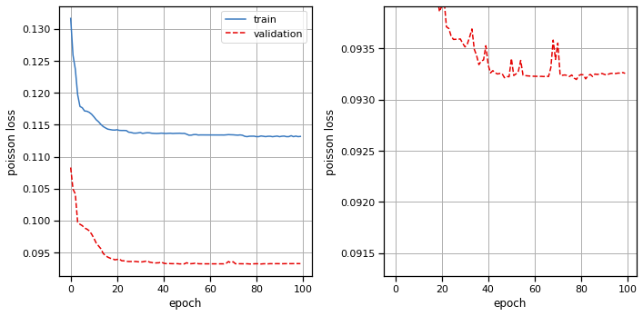
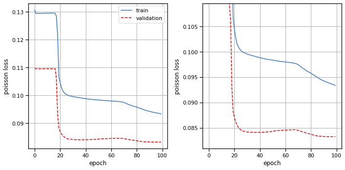
Plot the results

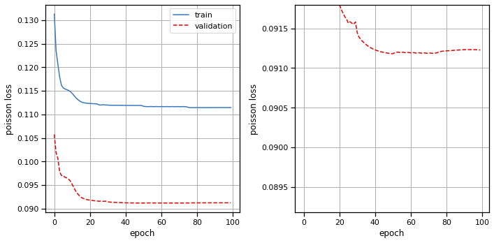
# Plot the training and validation curves
fig, axs = plt.subplots(1, 2, figsize=(10, 5))
axs[0].plot(train_losses, color=palette[0], label="train")
axs[0].plot(val_losses, color=palette[1], ls='--', label="validation")
axs[0].set_xlabel("epoch")
axs[0].set_ylabel("poisson loss")
axs[0].grid(True)
axs[0].legend(loc="upper right")

axs[1].plot(train_losses, color=palette[0], label="train")
axs[1].plot(val_losses, color=palette[1], ls='--', label="validation")
axs[1].set_xlabel("epoch")
axs[1].set_ylabel("poisson loss")
axs[1].set_ylim(top=val_losses[20])
axs[1].grid(True)

plt.tight_layout()

plot_stimulus_weights(lnp)

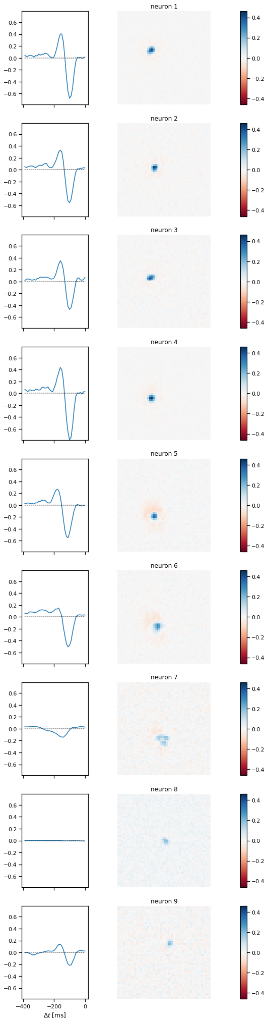
Problem 2d: [Short Answer] Interpret the results

How do the spatiotemporal filters relate to the STA from Problem 1c? Are they mathematically related?

---

Your answer here

Part 3: Fit a GLM with inter-neuron couplings

Image credit: Jonathan Pillow, Cosyne Tutorial 2018.

Now add inter-neuron couplings to the basic model above. For historical reasons, the LNP with inter-neuron couplings is what some neuroscientists call a GLM, even though they’re both instances of generalized linear models! Again, we’re just going to stick to the notation of McIntosh et al (2016) for this lab anyway.

The new model has activation,

\[ a_{t,n} = [\tilde{\mathbf{x}}_n \star \mathbf{v}_n]_t + \sum_{m=1}^N \sum_{d=1}^D y_{t-d,m} g_{m,n,d} \]

where \(\mathbf{G} \in \mathbb{R}^{N \times N \times D}\) is a tensor of coupling weights.

You can implement the activation using a convolution of \(\mathbf{Y}\) and \(\mathbf{G}\).

Note: as above, the coupling_conv will have a bias by default. Get rid of it. You don’t need it since there’s already a bias in the temporal_conv.

IMPORTANT: Make sure your output only depends on spike counts up to but not including time \(t\)!!

Problem 3a: Implement the coupled model

class GLM(nn.Module):
    def __init__(self,
                 num_neurons=num_neurons,
                 height=height,
                 width=width,
                 max_delay=40,
                 initial_bias=0.05,
                 mean_function=torch.exp):
        super(GLM, self).__init__()
        self.num_neurons = num_neurons
        self.height = height
        self.width = width
        self.max_delay = max_delay
        self.mean_function = mean_function

        ###
        # YOUR CODE BELOW
        self.spatial_conv = nn.Linear(...)
        self.temporal_conv = nn.Conv1d(...)
        self.coupling_conv = nn.Conv1d(...)
        ###

        # Initialize the bias
        torch.nn.init.constant_(self.temporal_conv.bias, 
                                torch.log(torch.tensor(initial_bias)))

    def forward(self, stimulus, spikes):
        """
        stimulus: num_frames x height x width
        spikes: num_frames x num_neurons
        
        returns: num_frames x num_neurons tensor of expected spike counts
        """
        x, y = stimulus, spikes

        ###
        # YOUR CODE BELOW
        rate = ...
        ###

        return 1e-4 + rate

# Construct a coupled GLM model with random initial weights.
torch.manual_seed(0)
glm = GLM(num_neurons=9).to(device)
check_model_outputs(glm)

Problem 3b: Implement a regularizer for the coupled GLM weights

Put an \(\ell_2\) penalty on the weights of the spatial_conv, temporal_conv, and coupling_conv. No need to regularize the bias. Scale the regularization by \(\alpha\).

def glm_regularizer(model, alpha=1e-3):
    """
    Implement an \ell_2 penalty on the norm of the model weights,
    as described above.

    model: GLM instance
    alpha: scaling parameter for the \ell_2 penalty.
    """
    ###
    # YOUR CODE BELOW
    reg = ...
    ###

    return reg

Fit the GLM model with couplings between neurons.

# Construct a coupled GLM model with random initial weights.
torch.manual_seed(0)
glm = GLM().to(device)

# Fit the model
print("Training coupled GLM. This should take about 2-4 minutes...")
train_losses, val_losses = \
    train_model(glm, 
                train_dataset, 
                val_dataset, 
                poisson_loss,
                glm_regularizer)

Training coupled GLM. This should take about 2-4 minutes...

Plot the results

# Plot the training and validation curves
fig, axs = plt.subplots(1, 2, figsize=(10, 5))
axs[0].plot(train_losses, color=palette[0], label="train")
axs[0].plot(val_losses, color=palette[1], ls='--', label="validation")
axs[0].set_xlabel("epoch")
axs[0].set_ylabel("poisson loss")
axs[0].grid(True)
axs[0].legend(loc="upper right")

axs[1].plot(train_losses, color=palette[0], label="train")
axs[1].plot(val_losses, color=palette[1], ls='--', label="validation")
axs[1].set_xlabel("epoch")
axs[1].set_ylabel("poisson loss")
axs[1].set_ylim(top=val_losses[20])
axs[1].grid(True)

plt.tight_layout()

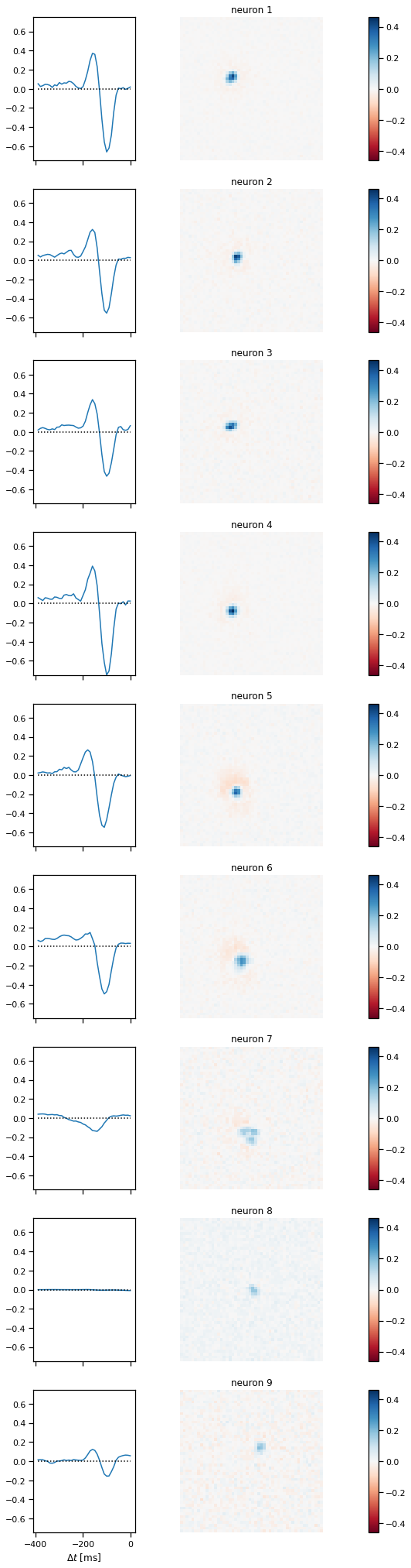
plot_stimulus_weights(glm)

plot_coupling_weights(glm)

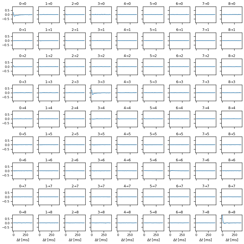
Problem 3c: [Short Answer] Interpret the results

Did adding the coupling weights change the spatiotemporal stimulus filters in any perceptible way? Do you see any interesting structure in the coupling weights? What other regularization strategies could you have applied to the coupling weights?

Your answer here

Part 4: Convolutional neural network model

Image credit: McIntosh et al (NeurIPS, 2016).

Finally, we’ll implement a convolutional neural network like the one proposed in McIntosh et al (2016). (See above.) We’ll make some slight modifications though, so that the model doesn’t take so long to fit.

Problem 4a: Implement the convolutional model

Implement the following model:

1. Apply a rank-1 spatiotemporal filter to the video:

   a. First convolve with 2D receptive fields of size rf_size_1 and num_subunits_1 output channels. You do not need to pad the edges since the neurons respond primarily to the center of the video. Your output should be T x N1 x H1 x W1 where T is the number of frames, N1 is the number of subunits, and H1,W1 are the height and width after 2D convolution without padding.

   b. Then convolve each subunit and pixel with a temporal filter, to get another T x N1 x H1 x W1 output.

   c. Apply a rectifying nonlinearity (F.relu).

2. Spatial convolution and mixing

   a. Apply a spatial convolution of size rf_size_2 with num_subunits_2 output channels. This layer mixes the subunits from the first layer to obtain a representation that is, hopefully, somewhat similar to that of intermediate cells in the retina.

   b. Apply another rectifying nonlinearity (F.relu). The output should be T x N2 x H2 x W2 where N2 is the number of subunits in the second layer and H2,W2 are the size of the image after convolution without padding.

3. Predict expected spike counts

   a. Apply a linear read-out to the N2 x H2 x W2 representation and pass through the mean function to obtain a T x N tensor of expected spike counts, where N is the number of neurons.

Notes: The modifications we made are

• We used slightly larger receptive field sizes. This actually speeds things up since, with valid padding, we end up with fewer “pixels” in subsequent layers.

• We used a smaller number of subunits (4/4 as opposed to 8/16). This is a smaller dataset (only 9 neurons) and we seemed to overfit with more layers.

• We use an exponential mean function to be consistent with the models above. Again, a softplus is more common in practice.

class CNN(nn.Module):
    def __init__(self,
                 num_neurons=num_neurons,
                 height=height,
                 width=width,
                 rf_size_1=21,
                 rf_size_2=15,
                 max_delay=40,
                 num_subunits_1=4,
                 num_subunits_2=4,
                 initial_bias=0.05,
                 mean_function=torch.exp):
        
        super(CNN, self).__init__()
        self.num_neurons = num_neurons
        self.height = height
        self.width = width
        self.max_delay = max_delay
        self.rf_size_1 = rf_size_1
        self.num_subunits_1 = num_subunits_1
        self.rf_size_2 = rf_size_2
        self.num_subunits_2 = num_subunits_2
        self.mean_function = mean_function
        
        ###
        # YOUR CODE BELOW
        self.spatial_conv = nn.Conv2d(...)
        self.temporal_conv = nn.Conv1d(...)
        self.layer2 = nn.Conv2d(...)
        self.layer3 = nn.Linear(...)
        ###

        # Initialize the bias
        torch.nn.init.constant_(self.layer3.bias, 
                                torch.log(torch.tensor(initial_bias)))
        
    def forward(self, stimulus, spikes=None):
        """
        stimulus: num_frames x height x width
        spikes: num_frames x num_neurons (unused by this model)
        
        returns: num_frames x num_neurons tensor of expected spike counts
        """
        x = stimulus
        
        ###
        # YOUR CODE BELOW
        rate = ...
        ###

        return 1e-4 + rate


torch.manual_seed(0)
cnn = CNN().to(device)
check_model_outputs(cnn)

Problem 4b: Regularize the weights

Put an \(\ell_2\) penalty on the weights of spatial_conv, temporal_conv, layer2, and layer3. Scale the regularize by \(\alpha\), as in the preceding sections. No need to regularize the biases. We found that a smaller value of \(\alpha\) was helpful, so here we default to 1e-5.

# Regularize the weights of the CNN
def cnn_regularizer(model, alpha=1e-5):
    """
    Implement an \ell_2 penalty on the norm of the model weights,
    as described above.

    model: CNN instance
    alpha: scaling parameter for the \ell_2 penalty.
    """
    ###
    # YOUR CODE BELOW
    reg = ...
    ###

    return reg

Fit the CNN model

torch.manual_seed(0)
cnn = CNN().to(device)

print("Fitting the CNN model. This should take about 10-20 minutes.")
train_losses, val_losses = \
    train_model(cnn, 
                train_dataset, 
                val_dataset,
                poisson_loss,
                cnn_regularizer)

Fitting the CNN model. This should take about 10-20 minutes.

Plot the results

# Plot the training and validation curves
fig, axs = plt.subplots(1, 2, figsize=(10, 5))
axs[0].plot(train_losses, color=palette[0], label="train")
axs[0].plot(val_losses, color=palette[1], ls='--', label="validation")
axs[0].set_xlabel("epoch")
axs[0].set_ylabel("poisson loss")
axs[0].grid(True)
axs[0].legend(loc="upper right")

axs[1].plot(train_losses, color=palette[0], label="train")
axs[1].plot(val_losses, color=palette[1], ls='--', label="validation")
axs[1].set_xlabel("epoch")
axs[1].set_ylabel("poisson loss")
axs[1].set_ylim(top=val_losses[10])
axs[1].grid(True)

plt.tight_layout()

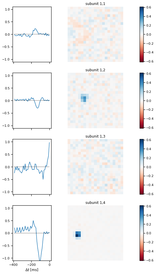
Plot the subunit weights for the CNN

First we’ll plot the spatiotemporal filters of the first layer of subunits.

plot_cnn_subunits_1(cnn)

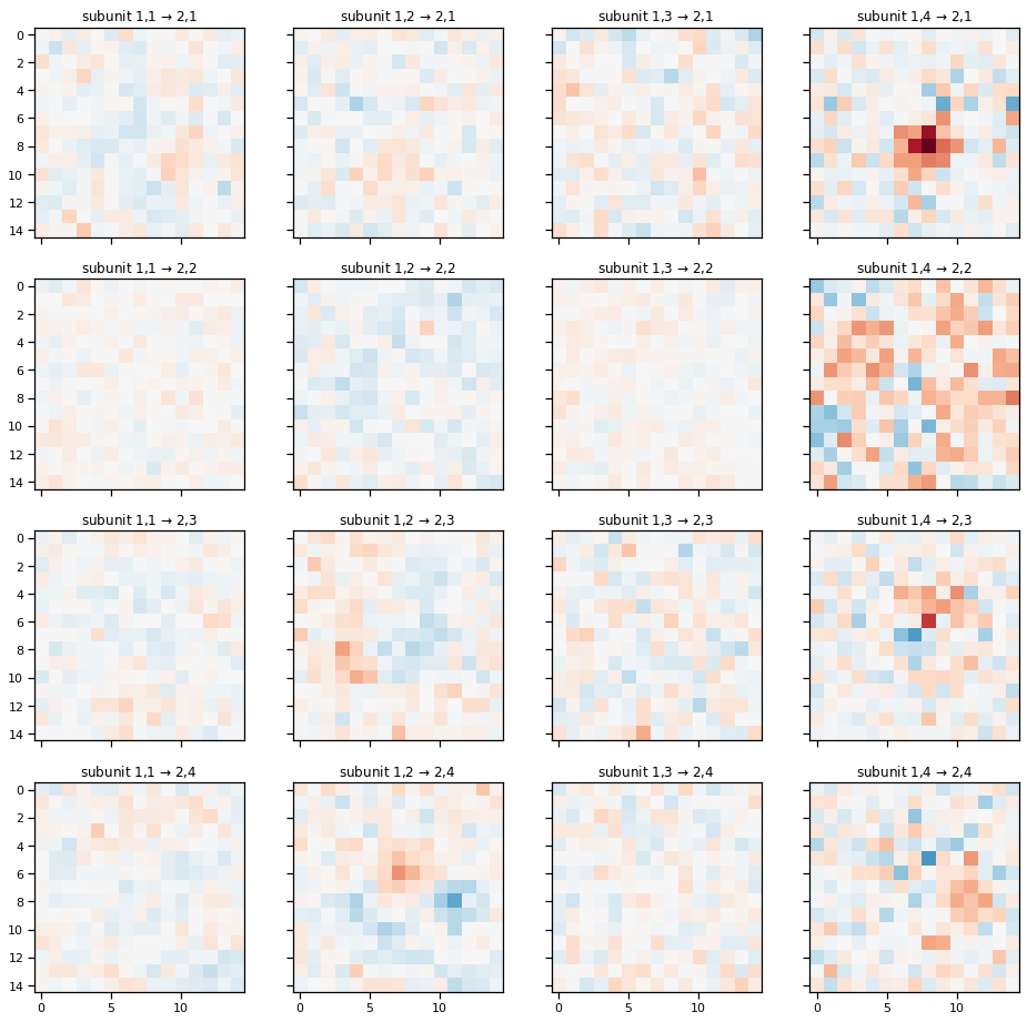
Plot the spatial weights for the second layer of subunits.

plot_cnn_subunits2(cnn)

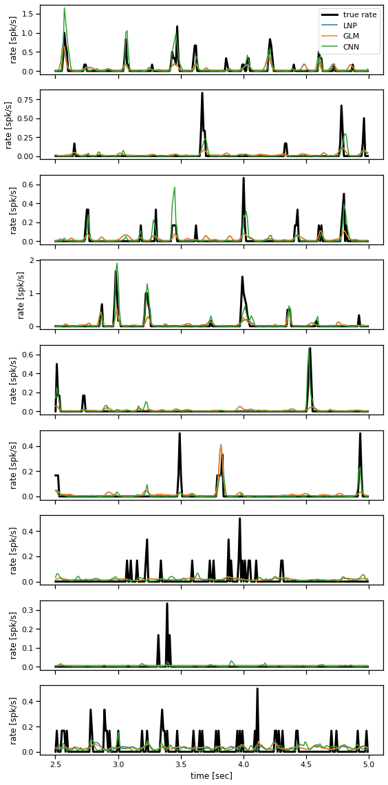
Problem 4c: Predict test firing rates

Finally, take the fitted models from Parts 2-4 and evaluate them on test data.

The test data consists of expected spike counts rather than spike counts. That’s because they showed the same visual stimulus many times and computed the average response. If our models are working well, they should output a similar firing rate in response to that same visual stimulus.

Note: technically the coupled GLM from Part 3 expects preceding spikes as input, but here we’ll give it the rates as input instead. (We don’t have test spikes to feed in.)

# Move the test stimulus and measured rates to the GPU
test_stimulus_cuda = test_stimulus.to(device).type(dtype) / 128.0
test_rates_cuda = test_rates.to(device)

###
# YOUR CODE BELOW
lnp_test_rates = ...
glm_test_rates = ...
cnn_test_rates = ...

# Plot a slice of the true and predicted firing rates
slc = slice(250, 500)
fig, axs = plt.subplots(num_neurons, 1, figsize=(8, 16), sharex=True)
for n in range(num_neurons):
    ...
###

plt.tight_layout()

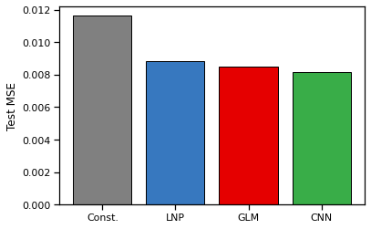
Problem 4d: Model comparison

Make a bar plot of the mean squared error between the true and predicted rates for each model. As a baseline, compute the mean squared error of a constant-rate model with rate equal to the expected spike count under the training data.

###
# YOUR CODE BELOW
mse_const = ...
mse_lnp = ...
mse_glm = ...
mse_cnn = ...
###

# Make a bar plot
plt.bar(0, mse_const, color='gray', ec='k')
plt.bar(1, mse_lnp, color=palette[0], ec='k')
plt.bar(2, mse_glm, color=palette[1], ec='k')
plt.bar(3, mse_cnn, color=palette[2], ec='k')
plt.xticks([0, 1, 2, 3], ["Const.", "LNP", "GLM", "CNN"])
plt.ylabel("Test MSE")

Text(0, 0.5, 'Test MSE')

Part 5: Discussion

You’ve now developed and fit three encoding models for these retinal ganglion cell responses, and hopefully you’ve developed some intuition for how these models work! Let’s end by discussing some of the decisions that go into building and checking these models.

Problem 5a

All three models were fit with a Poisson loss, which has unit dispersion. What is overdispersion of count data? Is this an issue here?

Your answer here

Problem 5b

The CNN was loosely motivated as an approximation to the layers of photoreceptors, bipolar cells, etc. that precede retinal ganglion cells. Of course, the actual circuitry is more complicated. What could you imagine adding to this model to make it more realistic?

Your answer here

Problem 5c

In our hands, the CNN outperformed the LNP and GLM. Though it’s tempting to just say the CNN is a more flexible model, notice that the CNN does not have coupling filters and it compresses the input substantially before the final read-out layer. Given the results above, what follow-up experiments would you do to further understand the root of these performance differences?

Your answer here

Problem 5d

We didn’t ask you to do a thorough hyperparameter search. If you were to do one, what are the key parameters you would vary to try to improve model performance?

Your answer here

Problem 5e

We fit all of these models to RGC responses to a binary white noise stimulus. Would you expect your results to change if the cells had been shown a movie with natural scenes instead?

Your answer here

Author contributions

Write a short paragraph describing how each team member contributed to this assignment.

Your answer here

Submission Instructions

Download your notebook in .ipynb format and use the following command to convert it to PDF

jupyter nbconvert --to pdf lab4_teamname.ipynb

If you’re using Anaconda for package management, you can install nbconvert with

conda install -c anaconda nbconvert

Upload your .pdf file to Gradescope.

Only one submission per team!