Probabilistic PCA

High-dimensional data often has far less intrinsic variation than the dimension $D$ would suggest. A class of students’ grade transcripts, or a collection of images, may vary along just a few underlying “axes.” Latent variable models make this intuition precise by positing that the high-dimensional observations $\mbx_n \in \reals^D$ are generated from a low-dimensional latent variable $\mbz_n \in \reals^M$ with $M \ll D$ .

In this chapter we study the simplest such models, where the relationship between $\mbz_n$ and $\mbx_n$ is linear and all distributions are Gaussian:

Principal Components Analysis (PCA): two classical optimization formulations and their connection to the eigenvectors of the sample covariance matrix
Probabilistic PCA (PPCA): PCA as the maximum likelihood solution to a Gaussian latent variable model, enabling Bayesian inference
Factor Analysis (FA): a generalization of PPCA with per-dimension noise variances
Other linear LVMs: Independent Components Analysis (ICA) and Probabilistic Canonical Correlation Analysis (PCCA)

Principal Components Analysis¶

Motivation¶

Suppose we observe grade transcripts $\{\mbx_n\}_{n=1}^N$ where $\mbx_n \in \reals^D$ is a vector of $D$ grades for student $n$ . We might want to:

Reduce dimensionality: are there a few axes of variation?
Visualize: embed the points in 2–3 dimensions for plotting.
Compress: summarize each student’s record compactly.

PCA addresses all three. There are two classical equivalent formulations.

Maximum Variance Formulation¶

Goal: project the data onto an $M$ -dimensional subspace while maximizing the variance of the projected data.

For $M = 1$ , let $\mbu_1 \in \reals^D$ be a unit vector defining the subspace. The projection of $\mbx_n$ is the scalar $\mbu_1^\top \mbx_n$ (the score or embedding). Its variance over the $N$ data points is:

\begin{align} \frac{1}{N} \sum_{n=1}^N \bigl[\mbu_1^\top \mbx_n - \mbu_1^\top \bar{\mbx}\bigr]^2 = \mbu_1^\top \mbS \mbu_1, \end{align}

(1)

where $\bar{\mbx} = \frac{1}{N}\sum_n \mbx_n$ is the sample mean and $\mbS = \frac{1}{N} \sum_n (\mbx_n - \bar{\mbx})(\mbx_n - \bar{\mbx})^\top$ is the sample covariance matrix.

Maximizing $\mbu_1^\top \mbS \mbu_1$ subject to $\|\mbu_1\|^2 = 1$ via a Lagrange multiplier gives $\mbS \mbu_1 = \lambda_1 \mbu_1$ , so $\mbu_1$ must be an eigenvector of $\mbS$ . Left-multiplying by $\mbu_1^\top$ shows the projected variance equals $\lambda_1$ , so we should choose the eigenvector with the largest eigenvalue.

More generally, the $M$ -dimensional principal subspace is spanned by the $M$ eigenvectors $\mbu_1, \ldots, \mbu_M$ with the largest eigenvalues $\lambda_1 \geq \cdots \geq \lambda_M$ .

Linear Autoencoder Formulation¶

Goal: find an orthogonal matrix $\mbW \in \reals^{D \times M}$ (with $\mbW^\top \mbW = \mbI_M$ ) that minimizes mean squared reconstruction error.

We encode as $\mbz_n = \mbW^\top (\mbx_n - \bar{\mbx})$ and decode as $\hat{\mbx}_n = \mbW \mbz_n + \bar{\mbx}$ . The loss is:

\begin{align} \mathcal{L}(\mbW) &= \frac{1}{N}\sum_{n=1}^N \|\mbx_n - \hat{\mbx}_n\|^2 = \Tr\bigl[(\mbI - \mbW\mbW^\top)\mbS(\mbI - \mbW\mbW^\top)\bigr] = \Tr[\mbS] - \Tr[\mbW^\top \mbS \mbW]. \end{align}

(2)

Minimizing $\mathcal{L}(\mbW)$ is equivalent to maximizing $\Tr[\mbW^\top \mbS \mbW] = \sum_{m=1}^M \lambda_m (\mbw_m^\top \mbu_m)^2$ , which is again solved by $\mbW = \mbU_M$ , the leading $M$ eigenvectors.

PCA and the Singular Value Decomposition¶

Let $\mbY = \frac{1}{\sqrt{N}} \mbX_c$ where $\mbX_c$ has rows $(\mbx_n - \bar{\mbx})^\top$ . Then $\mbY^\top \mbY = \mbS$ .

The SVD of $\mbY = \mbV \mbLambda^{1/2} \mbU^\top$ reveals:

Right singular vectors of $\mbY$ (columns of $\mbU$ ) = eigenvectors of $\mbS$ = principal components.
Squared singular values = eigenvalues $\lambda_1, \ldots, \lambda_D$ of $\mbS$ .

In practice, PCA is computed via SVD of $\mbY$ rather than by eigendecomposing $\mbS$ , since SVD is numerically more stable.

Explained Variance¶

The fraction of total variance captured by $M$ principal components is:

\begin{align} \text{variance explained} = \frac{\sum_{m=1}^M \lambda_m}{\sum_{d=1}^D \lambda_d}. \end{align}

(3)

A scree plot shows this quantity (per-component and cumulative) as a function of $M$ . Below we generate synthetic data from a rank-3 linear Gaussian model and visualize the scree plot.

# Generate synthetic data from a rank-3 linear Gaussian model
torch.manual_seed(305)
N, D, M_true = 300, 20, 3   # datapoints, features, true latent dims
W_true = torch.randn(D, M_true)         # D x M weight matrix
Z_true = torch.randn(N, M_true)         # N x M latent variables
σ2     = torch.tensor(0.5)              # noise variance
X = Z_true @ W_true.T + torch.sqrt(σ2) * torch.randn(N, D)

# Centre the data and compute PCA via SVD
μ  = X.mean(0)                          # sample mean, shape (D,)
Xc = X - μ                              # centred data, shape (N, D)
Y  = Xc / N**0.5                        # Y.T @ Y = sample covariance S
_, s, Vt = torch.linalg.svd(Y, full_matrices=False)
UM  = Vt.T                              # principal components, columns of UM
λ   = s**2                              # eigenvalues of S (variances)

fig, axs = plt.subplots(1, 2, figsize=(9, 4))

pct = 100 * λ / λ.sum()
axs[0].bar(range(1, D+1), pct.numpy(), color='steelblue', alpha=0.8)
axs[0].set_xlabel('Principal component')
axs[0].set_ylabel('Variance explained (%)')
axs[0].set_title('Per-component variance')

axs[1].plot(range(1, D+1), torch.cumsum(pct, 0).numpy(), 'o-', color='steelblue')
axs[1].axhline(90, color='r', ls='--', lw=1, label='90%')
axs[1].set_xlabel('Number of components')
axs[1].set_ylabel('Cumulative variance explained (%)')
axs[1].set_title('Scree plot')
axs[1].legend()

plt.tight_layout()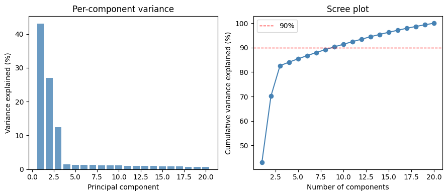

Probabilistic PCA¶

Model¶

The two classical formulations above cast PCA as an optimization problem. Probabilistic PCA (PPCA) instead defines a joint distribution over $\mbx_n$ and a latent variable $\mbz_n$ :

\begin{align} \mbz_n &\iid{\sim} \cN(\mbzero, \mbI_M) \\ \mbx_n \mid \mbz_n &\sim \cN(\mbW \mbz_n + \mbmu,\; \sigma^2 \mbI_D), \end{align}

(4)

where $\mbW \in \reals^{D \times M}$ are the loadings (analogous to the principal components), $\mbmu \in \reals^D$ is the mean, and $\sigma^2$ is an isotropic noise variance.

Equivalently, $\mbx_n = \mbW \mbz_n + \mbmu + \mbepsilon_n$ with $\mbepsilon_n \sim \cN(\mbzero, \sigma^2 \mbI_D)$ .

The marginal distribution of $\mbx_n$ is:

\begin{align} p(\mbx_n \mid \mbW, \mbmu, \sigma^2) = \cN(\mbx_n \mid \mbmu,\; \underbrace{\mbW\mbW^\top + \sigma^2 \mbI_D}_{\mbC}), \end{align}

(5)

a Gaussian with low-rank plus diagonal covariance — only $O(MD)$ parameters instead of $O(D^2)$ .

Maximum Likelihood Estimation¶

The marginal log-likelihood is:

\begin{align} \mathcal{L}(\mbW, \mbmu, \sigma^2) = -\frac{ND}{2}\log 2\pi - \frac{N}{2}\log|\mbC| - \frac{1}{2}\sum_{n=1}^N (\mbx_n - \mbmu)^\top \mbC^{-1} (\mbx_n - \mbmu). \end{align}

(6)

Tipping and Bishop (1999) showed the MLE has a closed form:

\begin{align} \mbmu_{\mathsf{ML}} &= \bar{\mbx}, \\ \mbW_{\mathsf{ML}} &= \mbU_M (\mbLambda_M - \sigma^2 \mbI)^{1/2} \mbR, \\ \sigma^2_{\mathsf{ML}} &= \frac{1}{D - M} \sum_{m=M+1}^D \lambda_m, \end{align}

(7)

where $\mbU_M$ contains the $M$ leading eigenvectors of the sample covariance $\mbS$ , $\mbLambda_M = \diag(\lambda_1, \ldots, \lambda_M)$ , and $\mbR \in \reals^{M \times M}$ is an arbitrary orthogonal matrix.

The weights are identifiable only up to orthogonal rotation — only the subspace spanned by $\mbU_M$ is uniquely determined. The MLE noise variance $\sigma^2_{\mathsf{ML}}$ is the average variance discarded in the trailing $D - M$ dimensions.

Posterior Distribution on Latent Variables¶

Given parameters $\mbW$ , $\mbmu$ , $\sigma^2$ , the posterior on $\mbz_n$ combines the Gaussian prior with the Gaussian likelihood:

\begin{align} p(\mbz_n \mid \mbx_n, \mbW, \mbmu, \sigma^2) = \cN(\mbz_n \mid \mbJ^{-1}\mbh_n,\; \mbJ^{-1}), \end{align}

(8)

where

\begin{align} \mbJ &= \mbI_M + \frac{1}{\sigma^2} \mbW^\top \mbW \in \reals^{M \times M}, \qquad \mbh_n = \frac{1}{\sigma^2} \mbW^\top (\mbx_n - \mbmu) \in \reals^M. \end{align}

(9)

Note that the posterior precision matrix $\mbJ$ is the same for all $n$ ; only the information vector $\mbh_n$ varies. The $M \times M$ system is much cheaper to invert than the $D \times D$ marginal covariance.

Zero-noise limit: as $\sigma^2 \to 0$ , the posterior mean converges to $(\mbW^\top \mbW)^{-1} \mbW^\top (\mbx_n - \mbmu)$ , the ordinary least-squares projection — identical to classical PCA (up to scaling).

# MLE for PPCA with M components
M_fit  = 3
UM_fit = Vt[:M_fit].T              # D x M leading principal components
ΛM     = torch.diag(λ[:M_fit])    # M x M eigenvalue matrix
σ2_ML  = λ[M_fit:].mean()         # MLE noise variance

# MLE weights (orthogonal rotation R = I)
W_ML = UM_fit @ (ΛM - σ2_ML * torch.eye(M_fit)).sqrt()

# Posterior on latent variables
J     = torch.eye(M_fit) + (1/σ2_ML) * W_ML.T @ W_ML   # M x M precision
Σz    = torch.linalg.inv(J)                              # M x M posterior cov
H     = Xc @ W_ML / σ2_ML                               # N x M info vectors
Z_hat = H @ Σz.T                                         # N x M posterior means

print(f'MLE noise variance σ²  = {σ2_ML:.3f}  (true = {σ2.item():.3f})')
print(f'Posterior covariance Σz:\n{Σz.numpy().round(3)}')

MLE noise variance σ²  = 0.483  (true = 0.500)
Posterior covariance Σz:
[[ 0.024  0.    -0.   ]
 [ 0.     0.038  0.   ]
 [-0.     0.     0.082]]

# Visualize the 2D posterior mean embedding
fig, ax = plt.subplots(figsize=(5, 5))
ax.scatter(Z_hat[:, 0].numpy(), Z_hat[:, 1].numpy(),
           c=Z_true[:, 0].numpy(), cmap='coolwarm', s=20, alpha=0.8)
ax.set_xlabel(r'$\hat{z}_1$ (posterior mean)')
ax.set_ylabel(r'$\hat{z}_2$ (posterior mean)')
ax.set_title('PPCA posterior mean embeddings')
plt.tight_layout()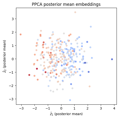

Gibbs Sampling for Probabilistic PCA¶

If we want a fully Bayesian treatment, we place a prior on the parameters. For simplicity assume $\mbmu = \mbzero$ (center the data first) and put:

\begin{align} p(\mbW, \sigma^2) = \chi^{-2}(\sigma^2 \mid \nu_0, \sigma_0^2) \prod_{d=1}^D \cN(\mbw_d \mid \mbzero,\, \tfrac{\sigma^2}{\kappa_0} \mbI_M), \end{align}

(10)

where $\mbw_d \in \reals^M$ is the $d$ -th row of $\mbW$ .

Complete conditional for each row $\mbw_d$ : combining the row prior with the $N$ likelihoods for the $d$ -th output gives a Gaussian:

\begin{align} p(\mbw_d \mid \{\mbz_n, \mbx_n\}, \sigma^2) = \cN(\mbw_d \mid \mbJ_d^{-1} \mbh_d,\; \mbJ_d^{-1}), \end{align}

(11)

where

\begin{align} \mbJ_d &= \frac{\kappa_0}{\sigma^2} \mbI_M + \frac{1}{\sigma^2} \sum_{n=1}^N \mbz_n \mbz_n^\top, \qquad \mbh_d = \frac{1}{\sigma^2} \sum_{n=1}^N x_{n,d}\, \mbz_n. \end{align}

(12)

Complete conditional for $\sigma^2$ : conjugate with the scaled inverse chi-squared family:

\begin{align} p(\sigma^2 \mid \{\mbz_n, \mbx_n\}, \mbW) &= \chi^{-2}(\sigma^2 \mid \nu_N, \sigma_N^2), \\ \nu_N &= \nu_0 + DM + DN, \\ \sigma_N^2 &= \frac{1}{\nu_N}\!\left[\nu_0 \sigma_0^2 + \kappa_0 \|\mbW\|_F^2 + \sum_{n=1}^N \|\mbx_n - \mbW \mbz_n\|^2\right]. \end{align}

(13)

Complete conditional for $\mbz_n$ : same as the PPCA posterior derived above.

Factor Analysis¶

Factor analysis (FA) relaxes the isotropic noise assumption of PPCA by allowing each output dimension to have its own noise variance:

\begin{align} \mbz_n &\iid{\sim} \cN(\mbzero, \mbI_M) \\ \mbx_n \mid \mbz_n &\sim \cN(\mbW \mbz_n + \mbmu,\; \diag(\mbsigma^2)), \end{align}

(14)

where $\mbsigma^2 = [\sigma_1^2, \ldots, \sigma_D^2]^\top$ . The marginal covariance is $\mbC = \mbW\mbW^\top + \diag(\mbsigma^2)$ — still low-rank plus diagonal, but with $D$ independent noise scales instead of one.

With the per-dimension prior:

\begin{align} p(\mbW, \mbsigma^2) = \prod_{d=1}^D \left[ \chi^{-2}(\sigma_d^2 \mid \nu_0, \sigma_0^2)\, \cN(\mbw_d \mid \mbzero,\, \tfrac{\sigma_d^2}{\kappa_0} \mbI_M) \right], \end{align}

(15)

the Gibbs updates for each $(\mbw_d, \sigma_d^2)$ pair are identical to those for PPCA but with $\sigma_d^2$ in place of the shared $\sigma^2$ . All rows are independent given $\{\mbz_n\}$ , so they can be updated in parallel.

Other Linear Latent Variable Models¶

Independent Components Analysis¶

ICA replaces the Gaussian latent prior with a product of non-Gaussian marginals:

\begin{align} \mbz_n &\iid{\sim} p(\mbz) = \prod_{m=1}^M p(z_m), \\ \mbx_n \mid \mbz_n &\sim \cN(\mbW \mbz_n + \mbmu,\; \diag(\mbsigma^2)). \end{align}

(16)

The non-Gaussian prior is essential: if $p(\mbz)$ were Gaussian, any correlation in $p(\mbz)$ could be absorbed into $\mbW$ , reducing the model to factor analysis. A common choice is a Laplace (heavy-tailed) prior, $p(z_m) \propto e^{-|z_m|}$ , which encourages the latent factors to be sparse.

ICA is widely used in signal processing (e.g., separating audio sources) and neuroscience.

Probabilistic Canonical Correlation Analysis¶

Suppose we observe two data modalities, $\mbx_n \in \reals^{D_x}$ and $\mby_n \in \reals^{D_y}$ . Probabilistic CCA posits:

\begin{align} \mbz_n^{(s)} &\iid{\sim} \cN(\mbzero, \mbI_{M_s}), & \mbz_n^{(x)} &\iid{\sim} \cN(\mbzero, \mbI_{M_x}), & \mbz_n^{(y)} &\iid{\sim} \cN(\mbzero, \mbI_{M_y}), \\ \mbx_n &\sim \cN(\mbW_{xx}\mbz_n^{(x)} + \mbW_{xs}\mbz_n^{(s)} + \mbmu_x,\; \sigma^2 \mbI_{D_x}), \\ \mby_n &\sim \cN(\mbW_{yy}\mbz_n^{(y)} + \mbW_{ys}\mbz_n^{(s)} + \mbmu_y,\; \sigma^2 \mbI_{D_y}). \end{align}

(17)

The shared latent variables $\mbz_n^{(s)}$ capture common structure across modalities; private variables $\mbz_n^{(x)}$ and $\mbz_n^{(y)}$ capture modality-specific variation.

Bach & Jordan, 2005 showed that the MLE recovers the classical CCA solution: the shared weights $\mbW_{xs}$ and $\mbW_{ys}$ correspond to the left and right singular vectors of the sample cross-correlation matrix $\diag(\mbS_{xx})^{-1/2} \mbS_{xy} \diag(\mbS_{yy})^{-1/2}$ .

Conclusion¶

This chapter developed a family of linear Gaussian latent variable models with progressively richer structure:

Model	Noise covariance	Latent prior
PPCA	$\sigma^2 \mbI$ (isotropic)	$\cN(\mbzero, \mbI)$
Factor analysis	$\diag(\mbsigma^2)$ (diagonal)	$\cN(\mbzero, \mbI)$
ICA	$\diag(\mbsigma^2)$	$\prod_m p(z_m)$ (non-Gaussian)
PCCA	$\sigma^2 \mbI$ (per modality)	shared + private Gaussians

Key takeaways:

PCA is the MLE for PPCA: the principal components are the leading eigenvectors of the sample covariance, computed efficiently via SVD.
The posterior on latent variables requires only inverting an $M \times M$ system (not $D \times D$ ), making inference tractable.
Gibbs sampling for PPCA / FA reduces to iterated Bayesian linear regressions — one per output dimension.
The non-Gaussian prior in ICA breaks the rotational indeterminacy of FA and enables recovery of independent source signals.