Expectation Maximization

The previous chapter introduced mixture models and two inference algorithms: K-Means (MAP via hard assignments) and a preview of EM (soft assignments via responsibilities). In this chapter we derive EM carefully and understand what it is optimising and why it works.

The key idea: rather than maximising the often-intractable marginal log-likelihood directly, EM iteratively constructs and maximises a tractable lower bound — the Evidence Lower Bound (ELBO) — by alternating between:

E-step: set the auxiliary distribution $q_n(z_n)$ to the posterior $p(z_n \mid \mbx_n, \mbtheta)$ , which makes the bound tight.
M-step: with $q$ fixed, maximise the ELBO over the parameters $\mbtheta$ , which increases the marginal log-likelihood.

Topics covered:

The marginal log-likelihood and why EM can outperform gradient ascent
Jensen’s inequality and the ELBO
KL divergence and the E-step optimality condition
Full derivation of E-step and M-step for Gaussian and general exponential-family mixture models
Code: tracking the ELBO and marginal log-likelihood across EM iterations

What is EM Optimising?¶

The Marginal Log-Likelihood¶

In the Bayesian mixture model, the parameters are $\mbtheta = (\mbpi, \{\mbtheta_k\})$ and each data point has a latent assignment $z_n$ . We want to find parameters that maximise the marginal log-likelihood (with a log-prior acting as regulariser):

\log p(\mbX, \mbtheta) = \log p(\mbtheta) + \sum_{n=1}^N \log \sum_{z_n=1}^K p(\mbx_n, z_n \mid \mbtheta).

(1)

For discrete mixtures with small $K$ we can evaluate this sum exactly, so in principle we could do gradient ascent on $\mbtheta$ .

Why prefer EM? EM exploits the structure of the model to obtain closed-form updates — no step-size tuning needed — and typically converges in far fewer iterations than gradient ascent on the marginal likelihood.

Review: Joint Distribution¶

The generative model gives:

p(\mbpi, \{\mbtheta_k\}, \{z_n, \mbx_n\}) = p(\mbpi \mid \mbalpha) \prod_{k=1}^K p(\mbtheta_k \mid \mbphi, \nu) \prod_{n=1}^N \prod_{k=1}^K \bigl[\pi_k\, p(\mbx_n \mid \mbtheta_k)\bigr]^{\mathbb{I}[z_n=k]}.

(2)

The Evidence Lower Bound (ELBO)¶

Jensen’s Inequality¶

Jensen’s inequality states that for any concave function $f$ and random variable $Y$ :

f\!\left(\mathbb{E}[Y]\right) \geq \mathbb{E}[f(Y)],

(3)

with equality if and only if $Y$ is constant (or $f$ is linear). Since $\log$ is concave, we have $\log \mathbb{E}[g(z)] \geq \mathbb{E}[\log g(z)]$ .

Deriving the ELBO¶

Introduce an auxiliary distribution $q_n$ over the discrete variable $z_n \in \{1,\ldots,K\}$ (any distribution with the same support):

\begin{aligned} \log p(\mbX, \mbtheta) &= \log p(\mbtheta) + \sum_{n=1}^N \log \sum_{z_n} q_n(z_n) \frac{p(\mbx_n, z_n \mid \mbtheta)}{q_n(z_n)} \\ &= \log p(\mbtheta) + \sum_{n=1}^N \log \mathbb{E}_{q_n}\!\left[\frac{p(\mbx_n, z_n \mid \mbtheta)}{q_n(z_n)}\right] \\ &\geq \log p(\mbtheta) + \sum_{n=1}^N \mathbb{E}_{q_n}\!\left[ \log p(\mbx_n, z_n \mid \mbtheta) - \log q_n(z_n) \right] \\ &\triangleq \mathcal{L}[\mbtheta, \mbq]. \end{aligned}

(4)

The bound $\mathcal{L}[\mbtheta, \mbq]$ is the ELBO. It holds for any choice of $\mbq = (q_1, \ldots, q_N)$ , and EM can be viewed as coordinate ascent on the ELBO over the joint space $(\mbtheta, \mbq)$ .

The KL Divergence and the E-Step¶

KL Divergence¶

The Kullback-Leibler divergence between distributions $q$ and $p$ is:

D_{\mathrm{KL}}(q(z) \| p(z)) = \sum_z q(z) \log \frac{q(z)}{p(z)} \geq 0,

(5)

with equality if and only if $q = p$ (almost everywhere). It is not symmetric, so it is not a metric.

The ELBO–KL Decomposition¶

We can rewrite the ELBO by adding and subtracting $\log p(z_n \mid \mbx_n, \mbtheta)$ inside the expectation:

\mathcal{L}[\mbtheta, \mbq] = \log p(\mbX, \mbtheta) - \sum_{n=1}^N D_{\mathrm{KL}}\!\bigl(q_n(z_n)\,\|\,p(z_n \mid \mbx_n, \mbtheta)\bigr).

(6)

Since KL $\geq 0$ , this confirms $\mathcal{L} \leq \log p(\mbX, \mbtheta)$ .

E-Step¶

Maximising $\mathcal{L}$ over $q_n$ (with $\mbtheta$ fixed) amounts to minimising the KL divergence to the posterior. The unique minimiser is:

\boxed{q_n^\star(z_n) = p(z_n \mid \mbx_n, \mbtheta).}

(7)

After the E-step, the KL terms vanish and the bound is tight:

\mathcal{L}[\mbtheta, \mbq^\star] = \log p(\mbX, \mbtheta).

(8)

For the Gaussian mixture model, setting $q_n = p(z_n \mid \mbx_n, \mbtheta)$ gives the responsibilities:

\omega_{nk} = q_n(z_n = k) = \frac{\pi_k\, \mathcal{N}(\mbx_n \mid \mbtheta_k, \mbI)}{\sum_{j=1}^K \pi_j\, \mathcal{N}(\mbx_n \mid \mbtheta_j, \mbI)}.

(9)

The M-Step¶

Gaussian Mixture Model¶

With $q_n$ fixed to the responsibilities $\{\omega_{nk}\}$ , the ELBO as a function of $\mbtheta_k$ (absorbing constants) is:

\mathcal{L}[\mbtheta, \mbq] \supseteq \sum_{k=1}^K \left[\mbphi^\top\mbtheta_k - \tfrac{\nu}{2}\mbtheta_k^\top\mbtheta_k\right] + \sum_{n=1}^N \sum_{k=1}^K \omega_{nk}\left[\mbx_n^\top \mbtheta_k - \tfrac{1}{2}\mbtheta_k^\top\mbtheta_k\right] + c.

(10)

Collecting terms for a single $\mbtheta_k$ :

\mathcal{L} \ni \mbphi_{N,k}^\top \mbtheta_k - \tfrac{\nu_{N,k}}{2}\mbtheta_k^\top \mbtheta_k,

(11)

where the pseudo-observations accumulate the soft sufficient statistics:

\mbphi_{N,k} = \mbphi + \sum_{n=1}^N \omega_{nk}\, \mbx_n, \qquad \nu_{N,k} = \nu + \sum_{n=1}^N \omega_{nk} = \nu + N_k.

(12)

Setting the gradient to zero:

\boxed{\mbtheta_k^\star = \frac{\mbphi_{N,k}}{\nu_{N,k}} = \frac{\mbphi + \sum_n \omega_{nk}\,\mbx_n}{\nu + N_k}.}

(13)

In the improper uniform prior limit ( $\mbphi \to \mathbf{0},\, \nu \to 0$ ): $\mbtheta_k^\star = \frac{1}{N_k}\sum_n \omega_{nk}\,\mbx_n$ — the responsibility-weighted sample mean.

The proportions update as $\pi_k = N_k / N$ .

EM as a Minorize-Maximize (MM) Algorithm¶

Each EM iteration:

E-step (minorize): construct the ELBO $\mathcal{L}[\mbtheta^{(t)}, \mbq]$ , which touches the marginal log-likelihood at $\mbtheta^{(t)}$ .
M-step (maximize): find $\mbtheta^{(t+1)} = \arg\max_{\mbtheta} \mathcal{L}[\mbtheta, \mbq^{(t)}]$ .

Because $\mathcal{L}[\mbtheta^{(t+1)}, \mbq^{(t)}] \geq \mathcal{L}[\mbtheta^{(t)}, \mbq^{(t)}]$ and $\mathcal{L} \leq \log p(\mbX, \mbtheta)$ , the marginal log-likelihood is guaranteed to increase (or stay the same) at every iteration.

EM for General Exponential-Family Mixtures¶

Generic M-Step¶

For an exponential-family likelihood $p(\mbx \mid \mbtheta_k) = h(\mbx)\exp\{\langle t(\mbx), \mbtheta_k\rangle - A(\mbtheta_k)\}$ with conjugate prior $p(\mbtheta_k \mid \mbphi, \nu) \propto \exp\{\langle \mbphi, \mbtheta_k\rangle - \nu A(\mbtheta_k)\}$ , the ELBO restricted to $\mbtheta_k$ is:

\mathcal{L} \ni \mbphi_{N,k}^\top \mbtheta_k - \nu_{N,k}\, A(\mbtheta_k), \quad \mbphi_{N,k} = \mbphi + \sum_n \omega_{nk}\, t(\mbx_n), \quad \nu_{N,k} = \nu + N_k.

(14)

Setting the gradient to zero: $\nabla A(\mbtheta_k) = \mbphi_{N,k}/\nu_{N,k}$ , so

\boxed{\mbtheta_k^\star = [\nabla A]^{-1}\!\left(\frac{\mbphi_{N,k}}{\nu_{N,k}}\right).}

(15)

Gradient of the Log Normalizer = Expected Sufficient Statistics¶

Why is $[\nabla A]^{-1}$ well defined? Differentiating the log normalizer:

\nabla A(\mbtheta_k) = \frac{\int h(\mbx)\,t(\mbx)\,e^{\langle t(\mbx),\mbtheta_k\rangle}\,d\mbx} {\int h(\mbx)\,e^{\langle t(\mbx),\mbtheta_k\rangle}\,d\mbx} = \mathbb{E}_{p(\mbx \mid \mbtheta_k)}[t(\mbx)].

(16)

So $\nabla A$ maps natural parameters to expected sufficient statistics. For a minimal exponential family this map is bijective, so the M-step reduces to: find the natural parameters that match the responsibility-weighted average of the sufficient statistics.

Model	$t(\mbx)$	$A(\mbtheta)$	M-step update $\mbtheta_k^\star$
Gaussian ( $\sigma^2=1$ )	$\mbx$	$\tfrac{1}{2}\|\mbtheta\|^2$	$\frac{1}{N_k}\sum_n \omega_{nk}\mbx_n$
Bernoulli	$x$	$\log(1+e^\theta)$	$\operatorname{sigmoid}^{-1}\!\left(\frac{\sum_n \omega_{nk} x_n}{N_k}\right) = \frac{\sum_n \omega_{nk} x_n}{N_k}$
Poisson	$x$	$e^\theta$	$\log\!\left(\frac{\sum_n \omega_{nk} x_n}{N_k}\right)$

torch.manual_seed(305)
N, K, D = 300, 3, 2

# True parameters
π_true = torch.tensor([0.3, 0.4, 0.3])
μ_true = torch.tensor([[-3., -1.], [1., 3.], [3., -2.]])
z_true = dist.Categorical(π_true).sample((N,))
x = μ_true[z_true] + torch.randn(N, D)


def em_gmm(x, K, num_iters=40, seed=0):
    """EM for isotropic-unit-variance GMM, tracking ELBO and marginal LL.

    At each iteration we record:
      elbo_E  -- ELBO right after the E-step  (equals marginal LL)
      ll_E    -- marginal log-likelihood after E-step  (= elbo_E)
      elbo_M  -- ELBO right after the M-step  (≤ new marginal LL)
      ll_M    -- marginal log-likelihood after M-step
    """
    torch.manual_seed(seed)

    # Initialise centroids by picking K random data points
    μ = x[torch.randperm(len(x))[:K]].clone().float()
    π = torch.ones(K) / K

    def e_step(μ, π):
        log_p = torch.stack(
            [dist.MultivariateNormal(μ[k], torch.eye(D)).log_prob(x) + π[k].log()
             for k in range(K)], dim=1)                  # (N, K)
        log_Z = torch.logsumexp(log_p, dim=1)            # (N,)
        ω = torch.exp(log_p - log_Z.unsqueeze(1))        # (N, K)
        return ω, log_Z.sum().item()

    def m_step(ω):
        N_k = ω.sum(0)
        π   = N_k / N
        μ   = (ω.T @ x) / N_k.unsqueeze(1)
        return μ, π

    def elbo(μ, π, ω):
        val = 0.0
        for k in range(K):
            lp = dist.MultivariateNormal(μ[k], torch.eye(D)).log_prob(x) + π[k].log()
            lq = torch.log(ω[:, k].clamp(min=1e-40))
            val += (ω[:, k] * (lp - lq)).sum().item()
        return val

    records = []
    for _ in range(num_iters):
        ω, ll_E = e_step(μ, π)
        elbo_E  = ll_E                     # bound is tight after E-step

        μ, π    = m_step(ω)
        _, ll_M = e_step(μ, π)             # recompute LL with updated params
        elbo_M  = elbo(μ, π, ω)            # ELBO with old q, new θ (may be loose)

        records.append(dict(elbo_E=elbo_E, ll_E=ll_E,
                            elbo_M=elbo_M, ll_M=ll_M))

    return μ, π, records


μ_em, π_em, records = em_gmm(x, K=3, num_iters=40)
print('Final means:')
for k in range(K):
    print(f'  k={k}: {μ_em[k].numpy().round(2)}')

Final means:
  k=0: [ 2.95 -2.  ]
  k=1: [-2.88 -0.93]
  k=2: [1.07 3.12]

iters     = list(range(1, len(records) + 1))
elbo_E    = [r['elbo_E'] for r in records]
ll_M      = [r['ll_M']   for r in records]
elbo_M    = [r['elbo_M'] for r in records]

fig, axes = plt.subplots(1, 2, figsize=(11, 4))

# ── Left: marginal LL vs ELBO per iteration ──────────────────────────────────
ax = axes[0]
ax.plot(iters, ll_M,   'o-', color='steelblue', label='Marginal LL  (after M-step)', lw=2, ms=4)
ax.plot(iters, elbo_E, 's--', color='tomato',
        label='ELBO = Marginal LL  (after E-step)', lw=1.5, ms=4)
ax.plot(iters, elbo_M, '^:', color='goldenrod',
        label='ELBO (after M-step, before next E-step)', lw=1.5, ms=4)
ax.set_xlabel('EM iteration')
ax.set_ylabel('Value')
ax.set_title('ELBO and marginal log-likelihood over EM')
ax.legend(fontsize=8)

# ── Right: zoom-in on first 10 iterations ────────────────────────────────────
ax = axes[1]
nshow = 10
ax.plot(iters[:nshow], ll_M[:nshow],   'o-', color='steelblue', lw=2, ms=5)
ax.plot(iters[:nshow], elbo_E[:nshow], 's--', color='tomato',   lw=1.5, ms=5)
ax.plot(iters[:nshow], elbo_M[:nshow], '^:', color='goldenrod', lw=1.5, ms=5)

# Annotate the gap between ELBO_M and LL_M on iteration 1
it = 0
ax.annotate('', xy=(iters[it], ll_M[it]), xytext=(iters[it], elbo_M[it]),
            arrowprops=dict(arrowstyle='<->', color='black', lw=1.5))
ax.text(iters[it] + 0.15, (ll_M[it] + elbo_M[it]) / 2,
        'KL gap', fontsize=8, va='center')

ax.set_xlabel('EM iteration')
ax.set_ylabel('Value')
ax.set_title('First 10 iterations (zoomed)')

plt.tight_layout()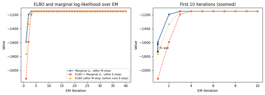

Conclusion¶

This chapter derived the EM algorithm from first principles:

	E-step	M-step
Action	Set $q_n^\star = p(z_n \mid \mbx_n, \mbtheta)$	Maximise ELBO over $\mbtheta$
Effect on ELBO	ELBO = marginal LL (bound tight)	ELBO increases
Effect on LL	No change (only $q$ changes)	Marginal LL increases

Key takeaways:

The ELBO lower-bounds the marginal log-likelihood; the gap is the sum of KL divergences $D_{\mathrm{KL}}(q_n \| p(z_n \mid \mbx_n, \mbtheta))$ .
The E-step closes this gap entirely by setting $q_n$ to the exact posterior.
The M-step increases the bound (and hence the likelihood) by finding better parameters given fixed responsibilities.
For exponential-family likelihoods, the M-step has a closed form: find natural parameters matching the responsibility-weighted sufficient statistics.
EM is guaranteed to monotonically increase the marginal log-likelihood and converges to a local maximum (global in some special cases).
Like K-Means, EM is sensitive to initialisation; random restarts or K-Means++ initialisation are recommended in practice.