Mixture Models - Overview

Real data rarely comes from a single homogeneous distribution. A dataset of cell transcriptomes likely contains multiple cell types; a scene image contains foreground objects against a background; a density can be multi-modal. Mixture models handle this by positing that each data point $\mbx_n$ was generated from one of $K$ latent components, with the component identity $z_n$ unobserved.

In this chapter we cover:

The mixture model: generative process, joint distribution, and exponential family components
MAP estimation by coordinate ascent: the celebrated K-Means algorithm
A preview of Expectation Maximization (EM), which uses soft assignments instead of hard ones (full derivation in the Expectation Maximization chapter)
Bayesian mixture models: placing priors on proportions and component parameters
The Dirichlet distribution as a conjugate prior on mixture proportions
Code: K-Means and EM on a simulated Gaussian mixture model

Motivation¶

Mixture models arise in many applications:

Clustering single-cell RNA-seq data: each cell belongs to one of several cell types, but the type is unobserved. See Kiselev et al., 2019 for a review of computational challenges.
Foreground/background segmentation: pixel colours in an image can be modelled as draws from one of two (or more) Gaussian components.
Density estimation: a mixture of Gaussians can approximate any smooth density arbitrarily well as $K \to \infty$ (a Gaussian mixture model is a universal density approximator).

Mixture Models¶

Notation¶

Symbol	Meaning
$N$	number of data points
$K$	number of mixture components
$\mbx_n \in \reals^D$	$n$ -th observation
$z_n \in \{1,\ldots,K\}$	latent component assignment of $\mbx_n$
$\mbtheta_k \in \reals^D$	mean of component $k$
$\mbpi \in \Delta_{K-1}$	component proportions

Generative Process¶

\begin{aligned} z_n &\iid{\sim} \operatorname{Categorical}(\mbpi) && n = 1, \ldots, N \\ \mbx_n &\sim \cN(\mbtheta_{z_n}, \mbI) && n = 1, \ldots, N \end{aligned}

(1)

Joint Distribution¶

The generative process implies the joint distribution:

p(\{z_n, \mbx_n\}_{n=1}^N; \mbtheta, \mbpi) = \prod_{n=1}^N \prod_{k=1}^K \left[\pi_k\, \cN(\mbx_n \mid \mbtheta_k, \mbI)\right]^{\mathbb{I}[z_n = k]}.

(2)

Summing over latent assignments gives the marginal likelihood:

p(\{\mbx_n\}_{n=1}^N; \mbtheta, \mbpi) = \prod_{n=1}^N \sum_{k=1}^K \pi_k\, \cN(\mbx_n \mid \mbtheta_k, \mbI).

(3)

torch.manual_seed(305)
N = 300   # number of data points
K = 3     # number of components
D = 2     # dimension

# True parameters
π_true = torch.tensor([0.3, 0.4, 0.3])
μ_true = torch.tensor([[-3., -1.], [1., 3.], [3., -2.]])

# Sample assignments then observations
z_true = dist.Categorical(π_true).sample((N,))        # shape (N,)
x = μ_true[z_true] + torch.randn(N, D)                # shape (N, D)

print(f'Data shape: {x.shape}')
print(f'Component counts: {[(z_true == k).sum().item() for k in range(K)]}')

Data shape: torch.Size([300, 2])
Component counts: [85, 122, 93]

fig, ax = plt.subplots(figsize=(5, 5))
for k in range(K):
    mask = z_true == k
    ax.scatter(x[mask, 0].numpy(), x[mask, 1].numpy(),
               color=palette[k], alpha=0.6, s=20, label=f'Component {k+1}')
    ax.scatter(*μ_true[k].numpy(), marker='*', s=250,
               color=palette[k], edgecolors='black', linewidths=0.5, zorder=5)
ax.set_xlabel(r'$x_1$')
ax.set_ylabel(r'$x_2$')
ax.set_title('Gaussian mixture model — true assignments')
ax.legend()
plt.tight_layout()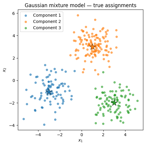

Two Inference Algorithms¶

Suppose we observe data $\{\mbx_n\}_{n=1}^N$ and want to infer the assignments $\{z_n\}_{n=1}^N$ and estimate the parameters $\{\mbtheta_k\}_{k=1}^K$ and proportions $\mbpi$ . We present two complementary approaches.

MAP Estimation and K-Means¶

Suppose we knew the cluster assignments $\{z_n\}$ . Then the maximum likelihood estimate of each component mean is simply the sample mean of its assigned points:

\hat{\mbtheta}_k = \frac{1}{N_k} \sum_{n=1}^N \mathbb{I}[z_n = k]\, \mbx_n, \qquad N_k = \sum_{n=1}^N \mathbb{I}[z_n = k].

(4)

Conversely, if we knew the means $\{\mbtheta_k\}$ , the MAP estimate of each assignment is the nearest centroid:

z_n^\star = \operatorname{arg\,min}_{k}\; \|\mbx_n - \mbtheta_k\|_2.

(5)

Alternating these two steps — with a uniform prior on $\mbtheta_k$ and equal proportions $\mbpi = \tfrac{1}{K}\mathbf{1}_K$ — is coordinate ascent on the joint MAP objective and yields the classic K-Means algorithm:

def kmeans(x, K, num_iters=50, seed=0):
    """K-Means via coordinate ascent (hard EM).

    Returns
    -------
    μ : (K, D) centroid matrix
    z : (N,) integer assignments
    obj_history : list of objective values (sum of squared distances)
    """
    torch.manual_seed(seed)
    N, D = x.shape

    # Initialise centroids by picking K random data points
    idx = torch.randperm(N)[:K]
    μ = x[idx].clone().float()

    obj_history = []
    z = torch.zeros(N, dtype=torch.long)

    for _ in range(num_iters):
        # Assignment step: z_n = argmin_k ||x_n - μ_k||
        dists = torch.cdist(x, μ)            # (N, K)
        z = dists.argmin(dim=1)              # (N,)

        # Update step: μ_k = mean of assigned points
        for k in range(K):
            mask = z == k
            if mask.sum() > 0:
                μ[k] = x[mask].mean(0)

        obj = sum(torch.norm(x[z == k] - μ[k], dim=1).pow(2).sum().item()
                  for k in range(K))
        obj_history.append(obj)

    return μ, z, obj_history

μ_km, z_km, obj_km = kmeans(x, K=3, num_iters=30)
print('K-Means centroids:')
for k in range(K):
    print(f'  k={k}: {μ_km[k].numpy().round(2)}')

K-Means centroids:
  k=0: [ 2.96 -2.01]
  k=1: [-2.87 -0.92]
  k=2: [1.08 3.12]

fig, axes = plt.subplots(1, 2, figsize=(10, 4))

# Left: K-means assignments
ax = axes[0]
for k in range(K):
    mask = z_km == k
    ax.scatter(x[mask, 0].numpy(), x[mask, 1].numpy(),
               color=palette[k], alpha=0.5, s=20)
    ax.scatter(*μ_km[k].numpy(), marker='*', s=300,
               color=palette[k], edgecolors='black', linewidths=0.8, zorder=5,
               label=f'Centroid {k+1}')
ax.set_xlabel(r'$x_1$')
ax.set_ylabel(r'$x_2$')
ax.set_title('K-Means assignments')
ax.legend(fontsize=9)

# Right: objective value
axes[1].plot(obj_km, 'o-', color='steelblue', markersize=4)
axes[1].set_xlabel('Iteration')
axes[1].set_ylabel(r'$\sum_n \|\mathbf{x}_n - \boldsymbol{\theta}_{z_n}\|^2$')
axes[1].set_title('K-Means objective')

plt.tight_layout()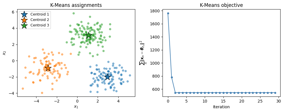

Expectation Maximization¶

K-Means makes hard assignments: each point belongs to exactly one cluster. The full Expectation Maximization (EM) algorithm instead computes soft assignments called responsibilities — the probability that data point $n$ belongs to component $k$ :

\omega_{nk} = \frac{\pi_k\, \mathcal{N}(\mbx_n \mid \mbtheta_k, \mbI)} {\sum_{j=1}^K \pi_j\, \mathcal{N}(\mbx_n \mid \mbtheta_j, \mbI)}.

(8)

The E-step computes responsibilities. The M-step updates parameters:

N_k = \sum_{n=1}^N \omega_{nk}, \qquad \pi_k = \frac{N_k}{N}, \qquad \mbtheta_k^\star = \frac{1}{N_k} \sum_{n=1}^N \omega_{nk}\, \mbx_n.

(9)

EM monotonically increases the marginal log-likelihood $\sum_n \log p(\mbx_n \mid \{\pi_k, \mbtheta_k\})$ . The next chapter develops EM in full generality.

def em_gmm(x, K, num_iters=50, seed=0):
    """EM for a Gaussian mixture model with identity covariances.

    Returns
    -------
    μ : (K, D) centroid matrix
    π : (K,) mixture weights
    ω : (N, K) responsibilities
    log_liks : list of marginal log-likelihoods
    """
    torch.manual_seed(seed)
    N, D = x.shape

    # Initialise with K-Means centroids
    μ, _, _ = kmeans(x, K, seed=seed)
    π = torch.ones(K) / K

    log_liks = []
    for _ in range(num_iters):
        # E-step: responsibilities
        log_p = torch.stack(
            [dist.MultivariateNormal(μ[k], torch.eye(D)).log_prob(x) + π[k].log()
             for k in range(K)], dim=1)          # (N, K)
        log_Z = torch.logsumexp(log_p, dim=1)    # (N,)
        ω = torch.exp(log_p - log_Z.unsqueeze(1))  # (N, K)
        log_liks.append(log_Z.sum().item())

        # M-step: update μ and π
        N_k = ω.sum(0)                            # (K,)
        π   = N_k / N
        μ   = (ω.T @ x) / N_k.unsqueeze(1)       # (K, D)

    return μ, π, ω, log_liks

μ_em, π_em, ω_em, ll_em = em_gmm(x, K=3, num_iters=50)
print('EM estimated means:')
for k in range(K):
    print(f'  k={k}: μ={μ_em[k].numpy().round(2)},  π={π_em[k]:.2f}')

EM estimated means:
  k=0: μ=[ 2.95 -2.  ],  π=0.31
  k=1: μ=[-2.88 -0.93],  π=0.28
  k=2: μ=[1.07 3.12],  π=0.41

fig, axes = plt.subplots(1, 3, figsize=(14, 4))

# Panel 1: EM soft assignments (colour = responsibility)
ax = axes[0]
colors = (ω_em.numpy()[:, :, None] * torch.tensor([palette[k] for k in range(K)])
                                        .numpy()[None, :, :]).sum(1)  # weighted RGB mix
ax.scatter(x[:, 0].numpy(), x[:, 1].numpy(),
           c=colors, s=20, alpha=0.7)
for k in range(K):
    ax.scatter(*μ_em[k].numpy(), marker='*', s=300,
               color=palette[k], edgecolors='black', linewidths=0.8, zorder=5,
               label=f'Component {k+1}')
ax.set_xlabel(r'$x_1$')
ax.set_ylabel(r'$x_2$')
ax.set_title('EM soft assignments')
ax.legend(fontsize=9)

# Panel 2: K-Means vs EM centroids vs true
ax = axes[1]
ax.scatter(x[:, 0].numpy(), x[:, 1].numpy(), color='lightgray', s=10, alpha=0.5)
for k in range(K):
    ax.scatter(*μ_true[k].numpy(), marker='D', s=150,
               color=palette[k], edgecolors='black', linewidths=0.8,
               label='True' if k == 0 else '_', zorder=6)
    ax.scatter(*μ_km[k].numpy(), marker='^', s=150,
               color=palette[k], edgecolors='gray', linewidths=0.8,
               label='K-Means' if k == 0 else '_', zorder=5)
    ax.scatter(*μ_em[k].numpy(), marker='*', s=250,
               color=palette[k], edgecolors='black', linewidths=0.8,
               label='EM' if k == 0 else '_', zorder=7)
ax.set_xlabel(r'$x_1$')
ax.set_ylabel(r'$x_2$')
ax.set_title('Centroids: True (◆) vs K-Means (▲) vs EM (★)')
ax.legend(fontsize=9)

# Panel 3: EM log-likelihood
axes[2].plot(ll_em, 'o-', color='steelblue', markersize=4)
axes[2].set_xlabel('Iteration')
axes[2].set_ylabel(r'$\sum_n \log p(\mathbf{x}_n)$')
axes[2].set_title('EM marginal log-likelihood')

plt.tight_layout()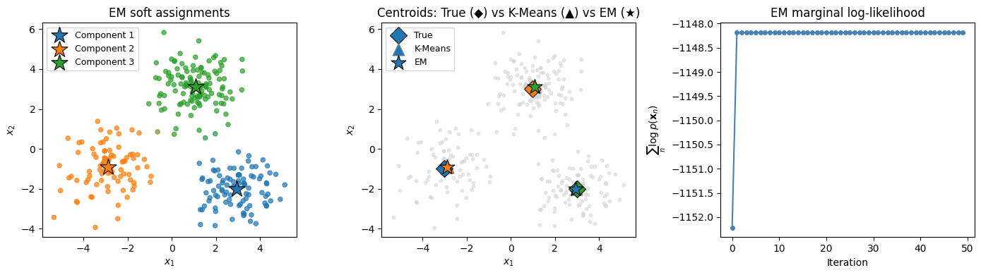

Exponential Family Mixture Models¶

The Gaussian mixture model is a special case of a broader family. Assume the emission distribution belongs to an exponential family:

p(\mbx \mid \mbtheta_k) = h(\mbx) \exp\!\left\{ \langle t(\mbx), \mbtheta_k \rangle - A(\mbtheta_k) \right\},

(10)

where $t(\mbx)$ are the sufficient statistics, $A(\mbtheta_k)$ is the log-normalizer, and $h(\mbx)$ is the base measure. The Gaussian case has $t(\mbx) = \mbx$ and $A(\mbtheta_k) = \tfrac{1}{2}\mbtheta_k^\top\mbtheta_k$ .

K-Means and EM extend naturally to any exponential family likelihood: the E-step (computing responsibilities) is unchanged, and the M-step for each component reduces to matching the responsibility-weighted sufficient statistics.

Bayesian Mixture Models¶

So far we have treated $\mbpi$ and $\{\mbtheta_k\}$ as fixed unknown parameters to be estimated. The Bayesian mixture model instead places priors on these quantities, enabling uncertainty quantification and regularisation via pseudo-counts.

Generative Process¶

\begin{aligned} \mbpi &\sim \operatorname{Dirichlet}(\mbalpha) \\ \mbtheta_k &\overset{\text{iid}}{\sim} p(\mbtheta \mid \mbphi, \nu) && k = 1, \ldots, K \\ z_n &\overset{\text{iid}}{\sim} \operatorname{Categorical}(\mbpi) && n = 1, \ldots, N \\ \mbx_n &\sim p(\mbx \mid \mbtheta_{z_n}) && n = 1, \ldots, N \end{aligned}

(11)

where $\mbalpha \in \reals_+^K$ is the Dirichlet concentration hyperparameter and $(\mbphi, \nu)$ are the hyperparameters of the conjugate prior on $\mbtheta_k$ .

Joint Distribution¶

p\!\left(\mbpi, \{\mbtheta_k\}, \{z_n, \mbx_n\}\right) = p(\mbpi \mid \mbalpha) \prod_{k=1}^K p(\mbtheta_k \mid \mbphi, \nu) \prod_{n=1}^N \prod_{k=1}^K \left[\pi_k\, p(\mbx_n \mid \mbtheta_k)\right]^{\mathbb{I}[z_n = k]}.

(12)

The M-step derived above continues to apply: the prior on $\mbtheta_k$ contributes $\nu$ pseudo-observations with pseudo-sufficient statistics $\mbphi$ , so the posterior natural parameters are $[\nabla A]^{-1}(\mbphi_{N,k}/\nu_{N,k})$ . Setting $\nu = 0$ and $\mbphi = \mathbf{0}$ recovers the MLE updates.

The Dirichlet Distribution¶

The Dirichlet distribution $\operatorname{Dirichlet}(\mbalpha)$ is the conjugate prior for the categorical / multinomial likelihood. It places a distribution over probability simplices $\mbpi \in \Delta_{K-1}$ :

p(\mbpi \mid \mbalpha) = \frac{\Gamma\!\left(\sum_k \alpha_k\right)}{\prod_k \Gamma(\alpha_k)} \prod_{k=1}^K \pi_k^{\alpha_k - 1}, \qquad \mbpi \in \Delta_{K-1}.

(13)

Interpretation of $\mbalpha$ :

$\alpha_k > 1$ : component $k$ is favoured (mode has $\pi_k > 1/K$ ).
$\alpha_k = 1$ : uniform prior over the simplex.
$\alpha_k < 1$ : sparse prior (probability mass concentrated near the corners of the simplex).
$\alpha_k = \alpha_0/K$ with $\alpha_0 \to 0$ : the symmetric sparse prior used in topic models.

For $K = 2$ the Dirichlet reduces to the Beta distribution $\operatorname{Beta}(\alpha_1, \alpha_2)$ over $\pi \in [0, 1]$ .

Posterior conjugacy: if $z_n \mid \mbpi \overset{\text{iid}}{\sim} \operatorname{Categorical}(\mbpi)$ and $\mbpi \sim \operatorname{Dirichlet}(\mbalpha)$ , then after observing counts $N_k = \sum_n \mathbb{I}[z_n = k]$ ,

\mbpi \mid \{z_n\} \sim \operatorname{Dirichlet}(\mbalpha + \mbN), \quad \mbN = (N_1, \ldots, N_K).

(14)

# Visualise Beta (K=2 Dirichlet) for several concentration parameters
fig, axes = plt.subplots(1, 4, figsize=(12, 3), sharey=False)

configs = [
    (0.5, 0.5, r'$\alpha_1=\alpha_2=0.5$ (sparse)'),
    (1.0, 1.0, r'$\alpha_1=\alpha_2=1$ (uniform)'),
    (2.0, 5.0, r'$\alpha_1=2,\, \alpha_2=5$'),
    (5.0, 2.0, r'$\alpha_1=5,\, \alpha_2=2$'),
]

π_vals = torch.linspace(0.01, 0.99, 300)
for ax, (a1, a2, title) in zip(axes, configs):
    log_p = (a1 - 1) * torch.log(π_vals) + (a2 - 1) * torch.log(1 - π_vals)
    p = torch.exp(log_p - log_p.max())
    ax.plot(π_vals.numpy(), p.numpy(), lw=2, color='steelblue')
    ax.set_xlabel(r'$\pi$')
    ax.set_title(title, fontsize=10)
    ax.set_xlim(0, 1)

axes[0].set_ylabel('density (unnormalised)')
plt.suptitle('Beta distribution (special case of Dirichlet, $K=2$)', fontsize=12)
plt.tight_layout()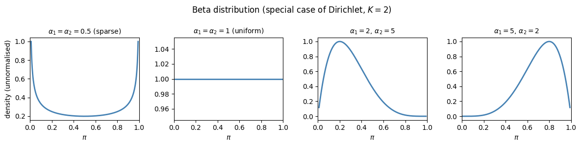

Conclusion¶

This chapter introduced mixture models and two algorithms for inference:

Algorithm	Assignment type	Objective
K-Means	Hard ( $z_n \in \{1,\ldots,K\}$ )	Joint MAP (mode of posterior)
EM	Soft ( $\omega_{nk} \in [0,1]$ )	Marginal likelihood

Key takeaways:

Mixture models are a natural framework for clustering and density estimation with discrete latent structure.
K-Means performs hard coordinate ascent on the joint MAP objective; each iteration is guaranteed to decrease the sum of squared distances.
EM replaces hard assignments with responsibilities (posterior probabilities), which smooths the objective and typically finds better solutions.
The Dirichlet distribution is the conjugate prior for mixture proportions; its concentration parameter $\mbalpha$ encodes how uniform or sparse the mixing weights should be.
Both algorithms are susceptible to local optima; multiple random restarts or a principled initialisation (e.g., K-Means++) are standard remedies.