This course is about probabilistic modeling and inference with high-dimensional data.
Throughout this course we will encounter data in many forms — vectors of measurements, images, documents, time series, spike trains — and our goal will be to build probabilistic models of that data and use them to reason about the world. Depending on the application, we might want to:
Predict: given features, estimate labels or outputs
Simulate: given partial observations, generate the rest
Summarize: given high-dimensional data, find low-dimensional factors of variation
Visualize: given high-dimensional data, find informative 2D/3D projections
Decide: given past actions and outcomes, determine the best future choice
Understand: identify what generative mechanisms gave rise to the data
A central theme is that probabilistic models provide a unified language for all of these tasks. By specifying a joint distribution over observed and latent variables, we can address prediction, simulation, and uncertainty quantification within a single coherent framework.
Box’s Loop
How should we go about building and using probabilistic models? A useful guiding framework is Box’s loop Blei, 2014, named after the statistician George Box (of “all models are wrong, but some are useful” fame). The loop has three stages:
Build: propose a probabilistic model — a joint distribution over data and parameters — that encodes your assumptions about how the data were generated.
Compute: perform inference to find the posterior distribution of the parameters given the observed data.
Critique: evaluate how well the model explains the data, check for systematic failures, and use those failures to motivate improvements.
Then repeat. Good probabilistic modeling is an iterative process: a simpler model helps us understand the data structure, and that understanding guides us toward richer, more accurate models.
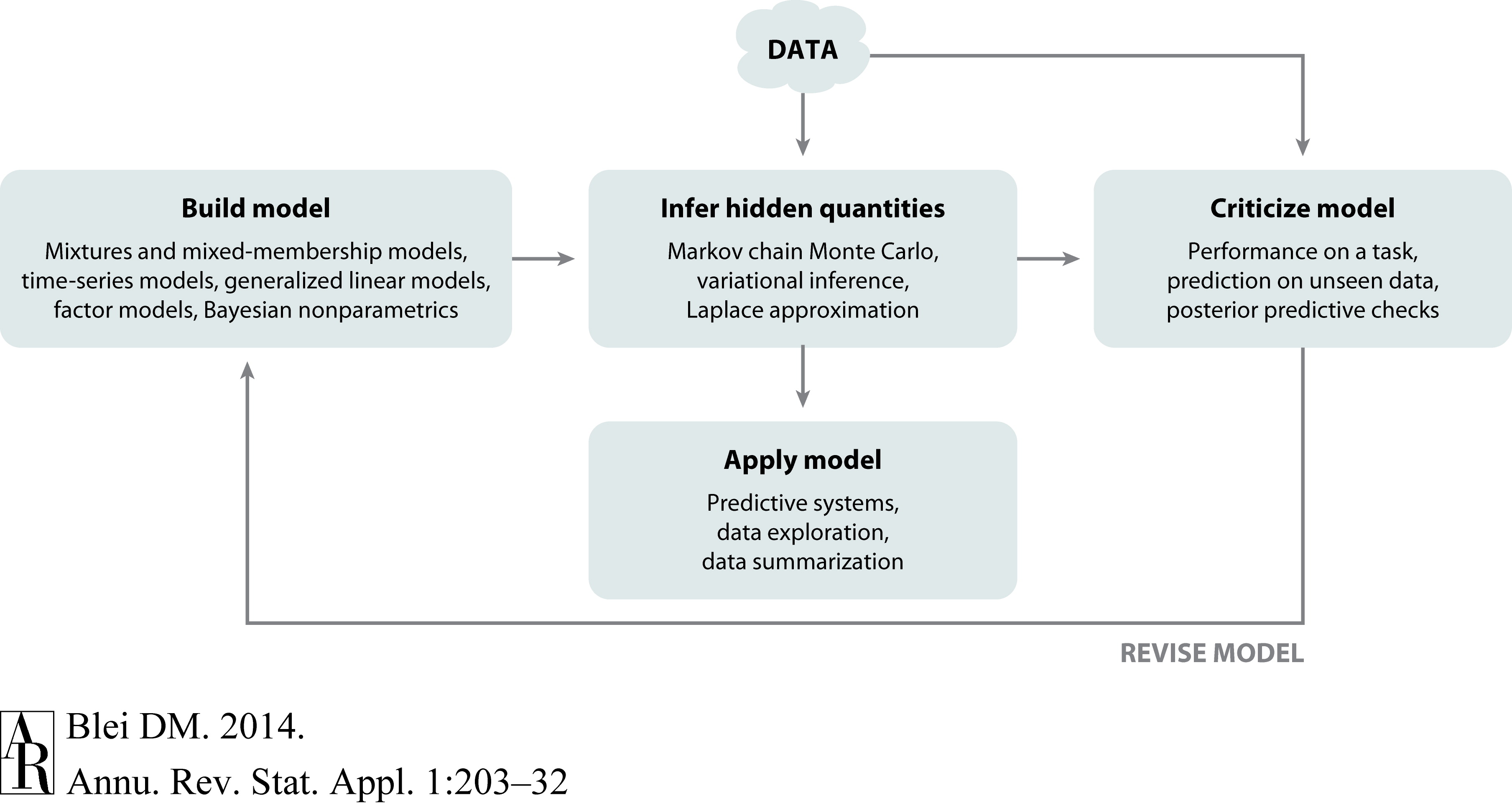
Figure 1:Box’s loop: the iterative cycle of model building, inference, and criticism. Figure from Blei, 2014.
The Bayesian Approach
The Bayesian approach to statistical modeling has three core components:
A model is a joint distribution of parameters and data ,
where is the prior distribution encoding beliefs about the parameters before seeing data, and is the likelihood of the data given parameters. The symbol denotes hyperparameters — parameters of the prior that we treat as fixed and known.
An inference algorithm computes the posterior distribution of parameters given data — a complete probabilistic description of what we have learned about after observing .
Model criticism and downstream tasks are based on posterior expectations — averages of quantities of interest under the posterior.
The fundamental formula connecting all three components is Bayes’ rule,
The marginal likelihood is the probability of the data averaged over all parameter values. It plays a key role in model comparison and hyperparameter selection, but computing it is often the hardest part — most of this course is about methods for dealing with this integral.
Notation. Throughout these notes: lowercase bold letters denote vectors (e.g., ); uppercase bold letters denote matrices (e.g., ); and regular characters denote scalars (e.g., ). We write for a dataset of observations.
TODO: Worked Example(s)
TODO: Project Description
Conclusion
This chapter introduced the Bayesian approach to probabilistic modeling. The core framework — prior, likelihood, posterior, and marginal likelihood — provides a unified language for learning from data under uncertainty. Box’s loop (build, compute, critique) captures the iterative nature of good probabilistic modeling: no model is final, and systematic criticism of model fit drives improvements. The hardest computational step is evaluating the marginal likelihood integral, and most of the course is devoted to algorithms that handle this challenge.
- Blei, D. M. (2014). Build, Compute, Critique, Repeat: Data Analysis with Latent Variable Models. Annual Review of Statistics and Its Application, 1, 203–232.