Bayesian Analysis of the Normal Distribution

import torch
from torch.distributions import Gamma, TransformedDistribution, Normal, StudentT
from torch.distributions.transforms import PowerTransform
import matplotlib.pyplot as plt
from matplotlib.cm import Blues

Normal Model with Unknown Mean¶

Let’s start with the simplest nontrivial Bayesian model to get a feel for how the machinery works.

We place a Gaussian prior on $\mu$ and model each score as an i.i.d. draw from a Gaussian with that mean:

\begin{align} \mu &\sim \cN(\mu_0, \sigma_0^2), \\ x_n \mid \mu &\iid{\sim} \cN(\mu, \sigma^2), \quad n = 1, \ldots, N. \end{align}

(1)

The hyperparameters are $\mbeta = (\mu_0, \sigma_0^2, \sigma^2)$ : the prior mean $\mu_0$ , prior variance $\sigma_0^2$ , and (known) data variance $\sigma^2$ . The prior variance $\sigma_0^2$ encodes how uncertain we are about the mean before seeing any data — a large $\sigma_0^2$ corresponds to a vague, spread-out prior.

Computing the Posterior¶

By Bayes’ rule, the posterior is proportional to the prior times the likelihood. Expanding the Gaussian densities,

\begin{align} p(\mu \mid \mbX; \mbeta) &\propto p(\mu; \mbeta) \prod_{n=1}^N p(x_n \mid \mu; \mbeta) \\ &= \cN(\mu; \mu_0, \sigma_0^2) \prod_{n=1}^N \cN(x_n; \mu, \sigma^2) \\ &\propto \exp \left\{ -\frac{(\mu - \mu_0)^2}{2 \sigma_0^2} \right\} \prod_{n=1}^N \exp \left\{ -\frac{(x_n - \mu)^2}{2 \sigma^2} \right\}. \end{align}

(2)

Since all factors are exponentials of quadratics in $\mu$ , the product is also an exponential of a quadratic in $\mu$ — which means the posterior is Gaussian. This is what it means for the Gaussian prior to be conjugate to the Gaussian likelihood.

To identify the posterior, we collect the terms quadratic and linear in $\mu$ in the exponent:

\begin{align} p(\mu \mid \mbX; \mbeta) &\propto \exp \left\{ -\frac{1}{2} J_N \mu^2 + h_N \mu \right\}, \end{align}

(3)

where we define the posterior precision and posterior information,

\begin{align} J_N = \frac{1}{\sigma_0^2} + \frac{N}{\sigma^2}, \qquad h_N = \frac{\mu_0}{\sigma_0^2} + \sum_{n=1}^N \frac{x_n}{\sigma^2}. \end{align}

(4)

The precision $J_N$ is simply the sum of the prior precision $1/\sigma_0^2$ and the total data precision $N/\sigma^2$ — information is additive. The information vector $h_N$ similarly sums contributions from the prior and each data point.

Completing the Square¶

The exponent $-\frac{1}{2} J_N \mu^2 + h_N \mu$ is a quadratic in $\mu$ . We can complete the square to convert it to the form $-\frac{1}{2\sigma_N^2}(\mu - \mu_N)^2 + \text{const}$ , where $\text{const}$ does not depend on $\mu$ . Specifically:

\begin{align} -\frac{1}{2} J_N \mu^2 + h_N \mu &= -\frac{J_N}{2}\left(\mu^2 - \frac{2 h_N}{J_N} \mu \right) = -\frac{J_N}{2}\left(\mu - \frac{h_N}{J_N}\right)^2 + \frac{h_N^2}{2 J_N}. \end{align}

(5)

Dropping the constant and recognizing $\sigma_N^2 = J_N^{-1}$ and $\mu_N = J_N^{-1} h_N = h_N / J_N$ , we find

\begin{align} p(\mu \mid \mbX; \mbeta) &= \cN(\mu \mid \mu_N, \sigma_N^2), \end{align}

(6)

where

\begin{align} \sigma_N^2 &= \left(\frac{1}{\sigma_0^2} + \frac{N}{\sigma^2}\right)^{-1}, \\[4pt] \mu_N &= \sigma_N^2 \left(\frac{\mu_0}{\sigma_0^2} + \frac{N \bar{x}}{\sigma^2}\right) = \frac{\sigma^2}{\sigma^2 + N\sigma_0^2}\, \mu_0 + \frac{N\sigma_0^2}{\sigma^2 + N\sigma_0^2}\, \mu_{\mathsf{ML}}, \end{align}

(7)

with $\bar{x} = \frac{1}{N}\sum_{n=1}^N x_n = \mu_{\mathsf{ML}}$ being the sample mean (and maximum likelihood estimate).

Interpreting the Posterior¶

The posterior mean $\mu_N$ is a weighted average of the prior mean $\mu_0$ and the MLE $\mu_{\mathsf{ML}}$ . The weights are determined by the relative precision of the prior versus the data. When $N$ is large, almost all weight goes to the data and $\mu_N \to \mu_{\mathsf{ML}}$ . When the prior is diffuse ( $\sigma_0^2 \to \infty$ , i.e., an uninformative prior), the prior precision vanishes and again $\mu_N \to \mu_{\mathsf{ML}}$ .

The posterior variance $\sigma_N^2$ follows a simpler pattern via the precision:

\begin{align} \frac{1}{\sigma_N^2} &= \frac{1}{\sigma_0^2} + \frac{N}{\sigma^2}. \end{align}

(8)

Each new observation contributes $1/\sigma^2$ of additional precision. As $N \to \infty$ , the posterior variance shrinks to zero — we become increasingly certain about $\mu$ . Under an uninformative prior ( $\sigma_0^2 \to \infty$ ), the posterior variance becomes $\sigma_N^2 = \sigma^2/N$ , the familiar sampling variance of the mean.

torch.manual_seed(305)

# Model hyperparameters and true parameter
μ0    = torch.tensor(0.0)
σ2_0  = torch.tensor(1.0)
σ2    = torch.tensor(1.0)

# Simulate data
N  = 20
μ  = Normal(μ0, torch.sqrt(σ2_0)).sample()
X  = Normal(μ, torch.sqrt(σ2)).expand([N]).sample()

# Compute posterior parameters
J_N     = 1 / σ2_0 + N / σ2
h_N     = μ0 / σ2_0 + X.sum() / σ2
μ_N     = h_N / J_N
σ2_N    = 1 / J_N

# Plot prior, likelihood, and posterior
prior = Normal(μ0, torch.sqrt(σ2_0))
lkhd  = Normal(μ, torch.sqrt(σ2))
post  = Normal(μ_N, torch.sqrt(σ2_N))
grid  = torch.linspace(-5, 5, 500)

fig, ax = plt.subplots()
ax.plot(grid, torch.exp(prior.log_prob(grid)),
        ':r', label=r"$p(\mu \mid \mu_0, \sigma_0^2)$")
ax.plot(grid, torch.exp(lkhd.log_prob(grid)),
        '-b', label=r"$p(x \mid \mu, \sigma^2)$")
ax.plot(grid, torch.exp(post.log_prob(grid)),
        '-', color='purple', label=r"$p(\mu \mid X, \mu_0, \sigma_0^2, \sigma^2)$")
ax.axvline(μ.item(), color='r', linestyle='--', lw=1, label=r"true $\mu$")
for n, x in enumerate(X):
    ax.axvline(x.item(), color='k', lw=0.5, alpha=0.4,
               label=r"$x_n$" if n == 0 else None)
ax.set_xlabel(r"$\mu$")
ax.set_ylabel("density")
ax.set_xlim(-5, 5)
ax.legend(fontsize=11)
ax.set_title("Prior, likelihood, and posterior for the Gaussian mean")
plt.tight_layout()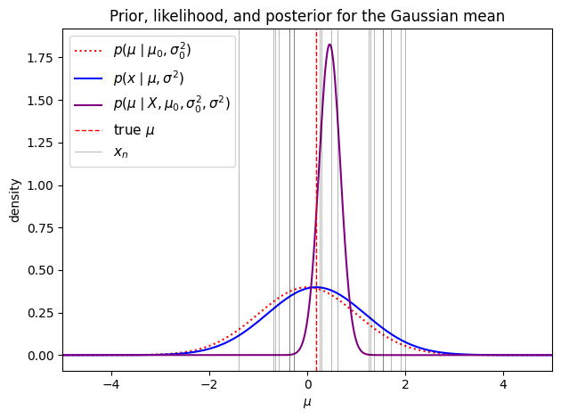

Normal Model with Unknown Precision¶

Now suppose the mean $\mu$ is known but the variance is not. Our calculations are slightly cleaner if we work with the precision $\lambda = 1/\sigma^2$ rather than the variance directly. In terms of the precision, the Gaussian density is,

\begin{align} p(x \mid \mu, \lambda) &= \left(\frac{\lambda}{2\pi}\right)^{\frac{1}{2}} \exp\left\{-\frac{\lambda}{2}(x - \mu)^2\right\}. \end{align}

(9)

What prior should we place on $\lambda$ ? We need a distribution on $\reals_+$ (since $\lambda > 0$ ), ideally one that is conjugate to the Gaussian likelihood. The chi-squared distribution fits the bill naturally.

The Chi-Squared Distribution¶

Let $z_1, \ldots, z_\nu \iid{\sim} \cN(0, 1)$ and define $\lambda = \sum_{i=1}^\nu z_i^2$ . Then $\lambda$ follows a chi-squared distribution with $\nu$ degrees of freedom,

\begin{align} \lambda \sim \chi^2(\nu), \end{align}

(10)

with pdf

\begin{align} \chi^2(\lambda; \nu) &= \frac{1}{2^{\nu/2} \Gamma(\nu/2)} \lambda^{\nu/2 - 1} e^{-\lambda/2}. \end{align}

(11)

This is a special case of the gamma distribution: $\chi^2(\nu) = \mathrm{Ga}(\nu/2,\, 1/2)$ using the rate parameterization. Its mean is $\E[\lambda] = \nu$ and its variance is $\Var[\lambda] = 2\nu$ .

The Scaled Chi-Squared Distribution¶

The standard chi-squared has mean $\nu$ , which grows with the degrees of freedom. For a prior over precision, it is more convenient to control the mean independently of the degrees of freedom. We do this by drawing from a scaled version: let $z_i \iid{\sim} \cN(0, \lambda_0)$ and define $\lambda = \frac{1}{\nu_0} \sum_{i=1}^{\nu_0} z_i^2$ (note the average rather than the sum). Then we say

\begin{align} \lambda \sim \chi^2(\nu_0, \lambda_0), \end{align}

(12)

where $\lambda_0 > 0$ is the scale parameter. Since $z_i = \sqrt{\lambda_0} \tilde{z}_i$ with $\tilde{z}_i \iid{\sim} \cN(0,1)$ , we have $\lambda = \frac{\lambda_0}{\nu_0} \sum_{i=1}^{\nu_0} \tilde{z}_i^2$ , so $\lambda = \frac{\lambda_0}{\nu_0} \tilde{\lambda}$ where $\tilde{\lambda} \sim \chi^2(\nu_0)$ . Using the fact that the gamma distribution is closed under multiplicative scaling, $\lambda \sim \mathrm{Ga}(\nu_0/2,\, \nu_0 / (2\lambda_0))$ , giving the pdf

\begin{align} \chi^2(\lambda; \nu_0, \lambda_0) &= \frac{\left(\frac{\nu_0}{2\lambda_0}\right)^{\nu_0/2}}{\Gamma(\nu_0/2)}\, \lambda^{\nu_0/2 - 1} \exp\!\left(-\frac{\nu_0 \lambda}{2\lambda_0}\right). \end{align}

(13)

The mean is $\E[\lambda] = \lambda_0$ regardless of $\nu_0$ , and the variance is $\Var[\lambda] = 2\lambda_0^2 / \nu_0$ . The parameter $\nu_0$ controls concentration: larger $\nu_0$ gives a tighter distribution around its mean $\lambda_0$ .

class ScaledChiSq(Gamma):
    """Scaled chi-squared distribution χ²(ν, λ).

    Equivalent to Ga(ν/2, ν/(2λ)) using the rate parameterisation.
    The mean is λ and the variance is 2λ²/ν.
    """
    def __init__(self, ν, λ):
        Gamma.__init__(self, ν / 2, ν / (2 * λ))
        self.ν = ν
        self.λ = λ


λ0   = torch.tensor(2.)
grid = torch.linspace(1e-3, 10, 200)
dofs = [2, 4, 6, 8, 10]

fig, ax = plt.subplots()
for i, ν in enumerate(dofs):
    chisq = ScaledChiSq(torch.tensor(float(ν)), λ0)
    ax.plot(grid, torch.exp(chisq.log_prob(grid)),
            label=r"$\chi^2({}, {})$".format(ν, int(λ0)),
            color=Blues(0.3 + 0.7 * i / (len(dofs) - 1)))

ax.legend(fontsize=12)
ax.set_xlabel(r"$\lambda$")
ax.set_ylabel(r"$p(\lambda)$")
ax.set_title(r"Scaled $\chi^2$ Distribution ($\lambda_0=2$, varying $\nu_0$)")
plt.tight_layout()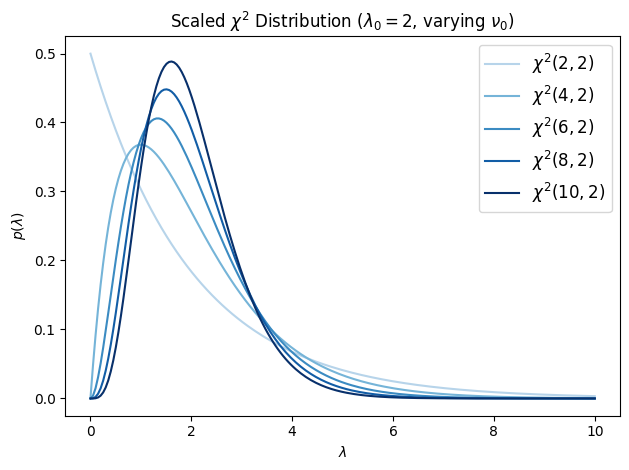

Conjugate Update¶

With the scaled chi-squared prior, the model is

\begin{align} \lambda &\sim \chi^2(\nu_0, \lambda_0), \\ x_n \mid \mu, \lambda &\iid{\sim} \cN(\mu, 1/\lambda), \quad n = 1, \ldots, N. \end{align}

(14)

The chi-squared distribution is conjugate to the Gaussian likelihood in $\lambda$ . Letting $\mbeta = (\mu, \nu_0, \lambda_0)$ , we compute:

\begin{align} p(\lambda \mid \mbX; \mbeta) &\propto \chi^2(\lambda; \nu_0, \lambda_0) \prod_{n=1}^N \cN(x_n; \mu, \tfrac{1}{\lambda}) \\ &\propto \lambda^{\nu_0/2 - 1} e^{-\nu_0 \lambda / (2\lambda_0)} \cdot \prod_{n=1}^N \lambda^{1/2} e^{-\frac{\lambda}{2}(x_n - \mu)^2} \\ &\propto \lambda^{(\nu_0 + N)/2 - 1} \exp\!\left(-\frac{\lambda}{2}\left[\frac{\nu_0}{\lambda_0} + \sum_{n=1}^N (x_n - \mu)^2\right]\right). \end{align}

(15)

This is another scaled chi-squared distribution, $p(\lambda \mid \mbX; \mbeta) = \chi^2(\lambda; \nu_N, \lambda_N)$ , where

\begin{align} \nu_N &= \nu_0 + N, \\ \lambda_N &= \nu_N \left(\frac{\nu_0}{\lambda_0} + \sum_{n=1}^N (x_n - \mu)^2\right)^{-1}. \end{align}

(16)

The posterior degrees of freedom grow by one per observation. As $\nu_0 \to 0$ (an uninformative prior), the posterior mean converges to $\lambda_N \to 1/\left(\frac{1}{N}\sum_n (x_n - \mu)^2\right)$ , the inverse of the sample variance — as expected.

Normal Model with Unknown Variance¶

Working with the precision is mathematically natural, but it can be more intuitive to parameterize the model in terms of the variance $\sigma^2 = 1/\lambda$ . If $\lambda \sim \chi^2(\nu_0, \lambda_0)$ , then the change-of-variables formula gives the distribution of $\sigma^2 = 1/\lambda$ :

\begin{align} p(\sigma^2 \mid \nu_0, \sigma_0^2) &= \left|\frac{\dif (1/\sigma^2)}{\dif \sigma^2}\right| \chi^2\!\left(\frac{1}{\sigma^2}; \nu_0, \frac{1}{\sigma_0^2}\right) \\ &= \frac{1}{(\sigma^2)^2} \cdot \frac{\left(\frac{\nu_0}{2\sigma_0^{-2}}\right)^{\nu_0/2}}{\Gamma(\nu_0/2)} \left(\frac{1}{\sigma^2}\right)^{\nu_0/2 - 1} \exp\!\left(-\frac{\nu_0}{2\sigma_0^2 \sigma^2}\right) \\ &= \frac{\left(\frac{\nu_0 \sigma_0^2}{2}\right)^{\nu_0/2}}{\Gamma(\nu_0/2)}\, (\sigma^2)^{-\nu_0/2 - 1} \exp\!\left(-\frac{\nu_0 \sigma_0^2}{2\sigma^2}\right) \\ &\triangleq \chi^{-2}(\sigma^2 \mid \nu_0, \sigma_0^2), \end{align}

(17)

where $\sigma_0^2 = 1/\lambda_0$ . This is the scaled inverse chi-squared distribution. It is a special case of the inverse gamma: $\chi^{-2}(\nu_0, \sigma_0^2) = \mathrm{IGa}(\nu_0/2,\, \nu_0 \sigma_0^2 / 2)$ .

The mean is $\E[\sigma^2] = \frac{\nu_0}{\nu_0 - 2} \sigma_0^2$ (for $\nu_0 > 2$ ) and the mode is $\frac{\nu_0}{\nu_0 + 2} \sigma_0^2$ . The parameter $\sigma_0^2$ is the prior “best guess” for the variance and $\nu_0$ controls how strongly that guess is held.

class ScaledInvChiSq(TransformedDistribution):
    """Scaled inverse chi-squared: χ⁻²(ν, σ²).

    Equivalent to IGa(ν/2, νσ²/2) using the rate parameterisation.
    The mean is σ²·ν/(ν-2) and the mode is σ²·ν/(ν+2).
    """
    def __init__(self, ν, σ2):
        base = Gamma(ν / 2, ν * σ2 / 2)
        TransformedDistribution.__init__(self, base, [PowerTransform(-1)])
        self.ν  = ν
        self.σ2 = σ2


σ2_0 = torch.tensor(2.)
grid  = torch.linspace(1e-3, 10, 200)
dofs  = [2, 4, 6, 8, 10]

fig, ax = plt.subplots()
for i, ν in enumerate(dofs):
    inv_chisq = ScaledInvChiSq(torch.tensor(float(ν)), σ2_0)
    ax.plot(grid, torch.exp(inv_chisq.log_prob(grid)),
            label=r"$\chi^{{-2}}({}, {})$".format(ν, int(σ2_0)),
            color=Blues(0.3 + 0.7 * i / (len(dofs) - 1)))

ax.legend(fontsize=12)
ax.set_xlabel(r"$\sigma^2$")
ax.set_ylabel(r"$p(\sigma^2)$")
ax.set_title(r"Scaled $\chi^{{-2}}$ Distribution ($\sigma_0^2=2$, varying $\nu_0$)")
plt.tight_layout()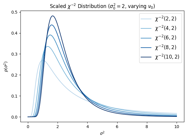

Parameterized in terms of the variance, the model is

\begin{align} \sigma^2 &\sim \chi^{-2}(\nu_0, \sigma_0^2), \\ x_n \mid \mu, \sigma^2 &\iid{\sim} \cN(\mu, \sigma^2). \end{align}

(18)

Normal Model with Unknown Mean and Variance¶

Finally, suppose both $\mu$ and $\sigma^2$ are unknown. We want a joint conjugate prior over $(\mu, \sigma^2)$ . The key insight is to write the prior as a product $p(\mu, \sigma^2) = p(\mu \mid \sigma^2) \, p(\sigma^2)$ : an inverse chi-squared prior on the variance, and conditional on the variance, a Gaussian prior on the mean whose variance scales with $\sigma^2$ . Specifically,

\begin{align} p(\mu, \sigma^2) &= \cN(\mu; \mu_0, \sigma^2 / \kappa_0) \, \chi^{-2}(\sigma^2; \nu_0, \sigma_0^2) \\ &\triangleq \mathrm{NIX}(\mu, \sigma^2; \mu_0, \kappa_0, \nu_0, \sigma_0^2). \end{align}

(20)

This is the normal-inverse-chi-squared (NIX) distribution — our first truly bivariate distribution. It has four hyperparameters: $\mu_0$ (prior mean), $\kappa_0$ (mean confidence, in pseudo-observations), $\nu_0$ (variance degrees of freedom), and $\sigma_0^2$ (prior variance scale).

The coupling $p(\mu \mid \sigma^2) = \cN(\mu_0, \sigma^2/\kappa_0)$ is crucial: the uncertainty in the mean is proportional to the variance. When $\sigma^2$ is large (we are uncertain about individual observations), we are also more uncertain about the mean. This dependence structure is what makes the NIX prior jointly conjugate.

torch.manual_seed(305)

μ0   = torch.tensor(0.)
κ0   = torch.tensor(1.0)
ν0   = torch.tensor(2.0)
σ2_0 = torch.tensor(2.0)

def sample_nix(μ0, κ0, ν0, σ2_0, n):
    σ2 = ScaledInvChiSq(ν0, σ2_0).sample(sample_shape=(n,))
    μ  = Normal(μ0, torch.sqrt(σ2 / κ0)).sample()
    return μ, σ2

# Evaluate the joint density on a grid
μ_grid, σ2_grid = torch.meshgrid(
    torch.linspace(-5, 5, 60),
    torch.linspace(1e-3, 10, 60),
    indexing='ij',
)
log_prob  = ScaledInvChiSq(ν0, σ2_0).log_prob(σ2_grid)
log_prob += Normal(μ0, torch.sqrt(σ2_grid / κ0)).log_prob(μ_grid)

fig, ax = plt.subplots()
cf = ax.contourf(μ_grid, σ2_grid, torch.exp(log_prob), 25)
μ_samp, σ2_samp = sample_nix(μ0, κ0, ν0, σ2_0, 25)
ax.scatter(μ_samp.numpy(), σ2_samp.numpy(),
           c='w', edgecolors='k', s=40, zorder=5)
ax.set_xlim(-5, 5)
ax.set_ylim(0, 10)
ax.set_xlabel(r"$\mu$")
ax.set_ylabel(r"$\sigma^2$")
ax.set_title(r"$\mathrm{{NIX}}(\mu_0={:.0f},\,\kappa_0={:.0f},\,\nu_0={:.0f},\,\sigma_0^2={:.0f})$".format(
    μ0, κ0, ν0, σ2_0))
plt.colorbar(cf, ax=ax, label=r"$p(\mu, \sigma^2)$")
plt.tight_layout()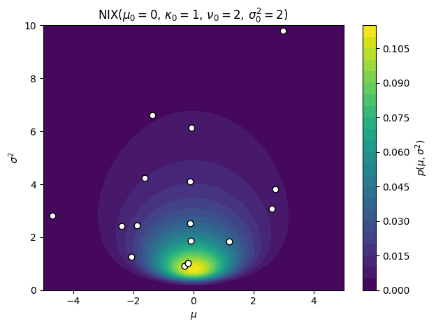

Posterior Update¶

With i.i.d. Gaussian observations $x_n \iid{\sim} \cN(\mu, \sigma^2)$ , the posterior under the NIX prior is again NIX:

Exercise

Show that $p(\mu, \sigma^2 \mid \mbX; \mbeta) = \mathrm{NIX}(\mu_N, \kappa_N, \nu_N, \sigma_N^2)$ , where

\begin{align} \kappa_N &= \kappa_0 + N, \\ \nu_N &= \nu_0 + N, \\ \mu_N &= \frac{\kappa_0 \mu_0 + \sum_{n=1}^N x_n}{\kappa_N} = \frac{\kappa_0}{\kappa_N}\mu_0 + \frac{N}{\kappa_N}\mu_{\mathsf{ML}}, \\ \sigma_N^2 &= \frac{1}{\nu_N}\left(\nu_0 \sigma_0^2 + \kappa_0 \mu_0^2 + \sum_{n=1}^N x_n^2 - \kappa_N \mu_N^2\right). \end{align}

(21)

Hint: write the prior and likelihood as exponentials of quadratics in $(\mu, 1/\sigma^2)$ and collect terms.

Just as in the known-variance case, $\mu_N$ is a weighted average of the prior mean and the sample mean. The posterior variance scale $\sigma_N^2$ can be rewritten as $\sigma_N^2 = \frac{1}{\nu_N}\left(\nu_0 \sigma_0^2 + \kappa_0 \mu_0^2 + \sum_n x_n^2 - \kappa_N \mu_N^2\right)$ , which combines the prior sum of squares with the data sum of squares, adjusted for the updated mean.

In the uninformative limit $\nu_0 \to 0$ , $\kappa_0 \to 0$ , the posterior parameters become $\nu_N = N$ , $\kappa_N = N$ , $\mu_N = \mu_{\mathsf{ML}}$ , and $\sigma_N^2 = \sigma^2_{\mathsf{ML}} = \frac{1}{N}\sum_n (x_n - \mu_{\mathsf{ML}})^2$ .

Posterior Marginals: Student’s t Distribution¶

What are the marginal distributions of $\mu$ and $\sigma^2$ under the NIX posterior? The marginal of $\sigma^2$ is straightforward — since $p(\mu, \sigma^2 \mid \mbX)$ is NIX, its $\sigma^2$ marginal is $\chi^{-2}(\nu_N, \sigma_N^2)$ .

The marginal of $\mu$ is more interesting. We integrate out $\sigma^2$ :

\begin{align} p(\mu \mid \mbX; \mbeta) &= \int p(\mu, \sigma^2 \mid \mbX; \mbeta) \dif \sigma^2 \\ &= \int \cN(\mu; \mu_N, \sigma^2 / \kappa_N) \, \chi^{-2}(\sigma^2; \nu_N, \sigma_N^2) \dif \sigma^2 \\ &= \mathrm{St}\!\left(\mu;\, \nu_N, \mu_N, \sigma_N^2 / \kappa_N\right), \end{align}

(22)

where $\mathrm{St}(\nu, \mu, \sigma^2)$ denotes the Student’s t distribution with $\nu$ degrees of freedom, location $\mu$ , and scale $\sigma^2$ , with density

\begin{align} \mathrm{St}(x; \nu, \mu, \sigma^2) &= \frac{\Gamma\!\left(\frac{\nu+1}{2}\right)}{\Gamma\!\left(\frac{\nu}{2}\right)} \frac{1}{\sqrt{\pi \nu \sigma^2}} \left[1 + \frac{(x - \mu)^2}{\nu \sigma^2}\right]^{-\frac{\nu+1}{2}}. \end{align}

(23)

Its mean is $\mu$ and its variance is $\frac{\nu}{\nu - 2}\sigma^2$ for $\nu > 2$ .

The Student’s t arises here because we are averaging a Gaussian over a random variance drawn from an inverse chi-squared distribution. When $\sigma^2$ is unknown and drawn from a broad distribution, the marginal distribution of $x$ has heavier tails than any single Gaussian — the extra uncertainty about the scale inflates the probability of large deviations. As $\nu \to \infty$ , the Student’s t converges to a Gaussian.

torch.manual_seed(305)

μ0   = torch.tensor(0.)
κ0   = torch.tensor(1.0)
ν0   = torch.tensor(2.0)
σ2_0 = torch.tensor(2.0)

# Analytical marginal p(μ) = St(ν0, μ0, σ2_0/κ0)
t_dist = StudentT(ν0, μ0, torch.sqrt(σ2_0 / κ0))

# Empirical samples from the NIX prior
σ2_samp = ScaledInvChiSq(ν0, σ2_0).sample(sample_shape=(10000,))
μ_samp  = Normal(μ0, torch.sqrt(σ2_samp / κ0)).sample()

μ_grid = torch.linspace(-6, 6, 200)
bins   = torch.linspace(-6, 6, 31)

fig, ax = plt.subplots()
ax.hist(μ_samp.numpy(), bins.numpy(), density=True,
        alpha=0.4, color='gray', ec='k', label='NIX samples')
ax.plot(μ_grid, torch.exp(t_dist.log_prob(μ_grid)),
        '-r', lw=2, label=r"$\mathrm{St}(\nu_0, \mu_0, \sigma_0^2/\kappa_0)$")
ax.plot(μ_grid,
        torch.exp(Normal(μ0, torch.sqrt(σ2_0 / κ0)).log_prob(μ_grid)),
        '--', color='purple', lw=2,
        label=r"$\mathcal{N}(\mu_0, \sigma_0^2/\kappa_0)$")
ax.legend(fontsize=11)
ax.set_xlim(-6, 6)
ax.set_xlabel(r"$\mu$")
ax.set_ylabel(r"$p(\mu)$")
ax.set_title("Student's t as the marginal of the NIX distribution")
plt.tight_layout()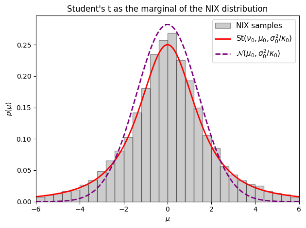

Posterior Credible Intervals¶

One of the main uses of the posterior is to construct credible intervals — Bayesian analogs of confidence intervals that have a direct probabilistic interpretation: $\mathcal{I}_\alpha$ is a $1-\alpha$ credible interval if $\Pr(\mu \in \mathcal{I}_\alpha \mid \mbX) = 1 - \alpha$ .

Under an uninformative prior, the posterior marginal is $\mu \mid \mbX \sim \mathrm{St}(N, \mu_{\mathsf{ML}}, \sigma^2_{\mathsf{ML}} / N)$ , and the central $1-\alpha$ credible interval is

\begin{align} \mathcal{I}_\alpha = \left[F_{\mathrm{St}}^{-1}\!\left(\tfrac{\alpha}{2} \,\Big|\, N, \mu_{\mathsf{ML}}, \frac{\sigma^2_{\mathsf{ML}}}{N}\right),\; F_{\mathrm{St}}^{-1}\!\left(1 - \tfrac{\alpha}{2} \,\Big|\, N, \mu_{\mathsf{ML}}, \frac{\sigma^2_{\mathsf{ML}}}{N}\right)\right], \end{align}

(24)

where $F_{\mathrm{St}}^{-1}$ is the quantile function of the Student’s t distribution.

Equivalently, note that the standardized quantity

\begin{align} t = \frac{\mu - \mu_{\mathsf{ML}}}{\sigma_{\mathsf{ML}} / \sqrt{N}} \;\Big|\; \mbX \;\sim\; \mathrm{St}(N, 0, 1), \end{align}

(25)

so testing whether a hypothesized value $\mu^*$ lies in $\mathcal{I}_\alpha$ is equivalent to checking whether the test statistic $t^* = (\mu^* - \mu_{\mathsf{ML}}) / (\sigma_{\mathsf{ML}} / \sqrt{N})$ satisfies $|t^*| \leq F_{\mathrm{St}}^{-1}(1 - \alpha/2 \mid N, 0, 1)$ .

This is structurally identical to the frequentist one-sample t-test, but with a different interpretation: instead of asking “how often would this test reject under repeated sampling?”, we ask “given the data we observed, how probable is it that $\mu$ lies outside this interval?” The Bayesian and frequentist answers happen to coincide numerically here (under the uninformative prior), but they represent fundamentally different epistemic claims.

Conclusion¶

This chapter developed Bayesian inference for the scalar Gaussian distribution from the ground up. The key takeaways are:

Conjugate priors make posterior inference tractable: the prior and posterior belong to the same family, so updating reduces to a simple update of hyperparameters.
The normal–inverse- $\chi^2$ prior is the natural conjugate for a Gaussian model with unknown mean and variance. Its two shape parameters $\nu_0$ and $\kappa_0$ can be interpreted as pseudo-observations informing the variance and mean estimates respectively.
The Student’s $t$ distribution emerges naturally as the marginal distribution of the mean after integrating out the unknown variance — heavier tails reflect our additional uncertainty about the scale.
Bayesian credible intervals have a direct probabilistic interpretation that differs conceptually from frequentist confidence intervals, even when the two coincide numerically under uninformative priors.