The Multivariate Normal Distribution

The multivariate normal (MVN) distribution — also called the multivariate Gaussian — is the workhorse of probabilistic machine learning. It is one of the few distributions in more than one dimension that we can work with analytically, and it arises naturally as the limiting distribution of sums of independent random vectors (the multivariate central limit theorem). Many of the models we study in this course are built from MVN distributions as building blocks.

In this lecture we cover:

The MVN distribution: generative story, density, marginals, conditionals, linear Gaussian models
Maximum likelihood estimation
The Wishart and inverse Wishart distributions
Bayesian estimation with a normal-inverse-Wishart (NIW) prior
Posterior marginals: the multivariate Student’s t distribution

import torch
from torch.distributions import Normal, MultivariateNormal, Wishart
import matplotlib.pyplot as plt


def plot_cov(Σ, μ=None, ax=None, **kwargs):
    """Visualize a 2D covariance matrix as a 1-σ ellipse."""
    D = Σ.shape[-1]
    μ = torch.zeros(D) if μ is None else μ
    λ_diag, U = torch.linalg.eigh(Σ)
    zs = torch.column_stack([
        torch.cos(torch.linspace(0, 2 * torch.pi, 50)),
        torch.sin(torch.linspace(0, 2 * torch.pi, 50))
    ])
    xs = (zs * torch.sqrt(λ_diag)) @ U.T
    ax = plt.axes(aspect=1) if ax is None else ax
    ax.plot(μ[0] + xs[:, 0], μ[1] + xs[:, 1], **kwargs)

Generative Story¶

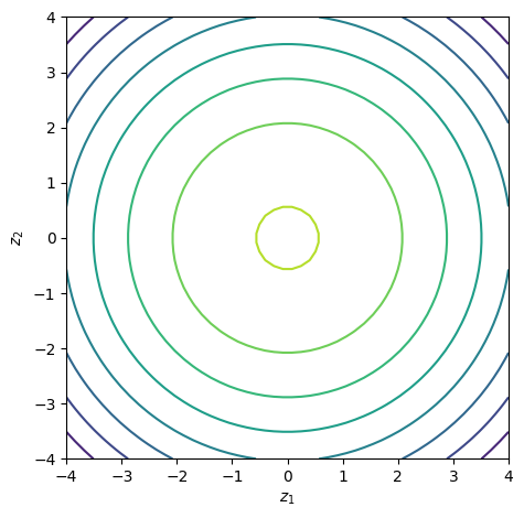
The cleanest way to understand the MVN is to build it up from scratch. Start with a vector of standard normal random variates, $\mbz = [z_1, \ldots, z_D]^\top$ , where each component is drawn independently,

\begin{align} z_d &\iid{\sim} \cN(0, 1) \quad \text{for } d = 1, \ldots, D. \end{align}

(1)

This $D$ -dimensional random variable is the simplest possible multivariate Gaussian, but it is not very interesting — all the coordinates are independent and have unit variance. Its joint density factors as a product of univariate Gaussians,

\begin{align} p(\mbz) &= \prod_{d=1}^D \cN(z_d \mid 0, 1) \\ &= \prod_{d=1}^D \frac{1}{\sqrt{2 \pi}} e^{-\frac{1}{2} z_d^2} \\ &= (2 \pi)^{-\frac{D}{2}} \exp\left\{ -\frac{1}{2} \sum_{d=1}^D z_d^2 \right\} \\ &= (2 \pi)^{-\frac{D}{2}} \exp\left\{ -\frac{1}{2} \mbz^\top \mbz \right\} \\ &\triangleq \cN(\mbz \mid \mbzero, \mbI). \end{align}

(2)

The last step recognizes this as a multivariate normal with zero mean and identity covariance. In $D=2$ dimensions, the contours of constant density are circles centered at the origin — hence the name spherical Gaussian.

torch.manual_seed(305)

z1, z2 = torch.meshgrid(
    torch.linspace(-4, 4, 50),
    torch.linspace(-4, 4, 50),
    indexing='ij',
)
log_p = Normal(0, 1).log_prob(z1) + Normal(0, 1).log_prob(z2)

fig, ax = plt.subplots()
ax.contour(z1, z2, log_p)
ax.set_xlabel(r"$z_1$")
ax.set_ylabel(r"$z_2$")
ax.set_aspect(1)
plt.tight_layout()

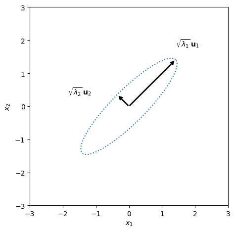
We can obtain more interesting joint distributions by linearly transforming this random vector. Let $\mbU$ be an orthogonal $D \times D$ matrix (so $\mbU^\top \mbU = \mbI$ ) whose columns are the eigenvectors of a desired covariance, and let $\mbLambda = \diag([\lambda_1, \ldots, \lambda_D])$ with $\lambda_d > 0$ be a diagonal matrix of eigenvalues. Define,

\begin{align} \mbx = \mbU \mbLambda^{\frac{1}{2}} \mbz. \end{align}

(3)

The matrix $\mbU$ rotates the coordinate axes, while $\mbLambda^{1/2}$ stretches each axis by a factor of $\sqrt{\lambda_d}$ . The result is a random vector whose variance along the $d$ -th eigenvector is $\lambda_d$ .

Density of the MVN¶

To find the density of $\mbx = \mbU \mbLambda^{1/2} \mbz$ , we apply the multivariate change-of-variables formula. Since $\mbx$ is an invertible linear function of $\mbz$ , with $\mbz = \mbLambda^{-1/2} \mbU^\top \mbx$ , the density transforms as,

\begin{align} p(\mbx) &= p(\mbz) \left| \frac{\dif \mbz}{\dif \mbx} \right| \\ &= p(\mbLambda^{-\frac{1}{2}} \mbU^\top \mbx) \, |\mbLambda^{-\frac{1}{2}} \mbU^\top| \\ &= (2 \pi)^{-\frac{D}{2}} \exp \left\{ -\frac{1}{2} \mbx^\top \mbU \mbLambda^{-1} \mbU^\top \mbx \right \} |\mbLambda^{-\frac{1}{2}}| \, |\mbU^\top| \\ &= (2 \pi)^{-\frac{D}{2}} \exp \left\{ -\frac{1}{2} \mbx^\top \mbU \mbLambda^{-1} \mbU^\top \mbx \right \} |\mbLambda|^{-\frac{1}{2}} \\ &= (2 \pi)^{-\frac{D}{2}} \exp \left\{ -\frac{1}{2} \mbx^\top \mbSigma^{-1} \mbx \right \} |\mbSigma|^{-\frac{1}{2}} \end{align}

(4)

where $\mbSigma = \mbU \mbLambda \mbU^\top$ . The key steps are: (i) the Jacobian of the linear map is the absolute value of the determinant of $\mbLambda^{-1/2} \mbU^\top$ ; (ii) since $\mbU$ is orthogonal, $|\mbU^\top| = 1$ ; and (iii) $|\mbLambda^{-1/2}| = |\mbLambda|^{-1/2}$ since $\mbLambda$ is diagonal.

Adding a translation so that $\mbx = \mbU \mbLambda^{\frac{1}{2}}\mbz + \mbmu$ for $\mbmu \in \reals^D$ , the same argument gives the general MVN density,

\begin{align} p(\mbx) &= (2\pi)^{-\frac{D}{2}} |\mbSigma|^{-\frac{1}{2}} \exp\left\{-\frac{1}{2} (\mbx - \mbmu)^\top \mbSigma^{-1} (\mbx - \mbmu) \right\} \triangleq \cN(\mbx \mid \mbmu, \mbSigma). \end{align}

(5)

This is the pdf of the multivariate normal (MVN) distribution with mean vector $\mbmu \in \reals^D$ and positive definite covariance matrix $\mbSigma \in \reals^{D \times D}$ .

The density depends on $\mbx$ only through the squared Mahalanobis distance,

\begin{align} \Delta^2 &= (\mbx - \mbmu)^\top \mbSigma^{-1} (\mbx - \mbmu). \end{align}

(6)

This is a generalization of the squared Euclidean distance that accounts for the scale and orientation of the distribution. Points $\mbx$ at equal Mahalanobis distance from $\mbmu$ lie on an ellipse whose axes are aligned with the eigenvectors of $\mbSigma$ and whose radii are proportional to $\sqrt{\lambda_d}$ .

torch.manual_seed(305)

# Eigenvectors (rotation by π/4)
θ  = torch.tensor(torch.pi / 4)
u1 = torch.stack([torch.cos(θ),  torch.sin(θ)])
u2 = torch.stack([-torch.sin(θ), torch.cos(θ)])
U  = torch.column_stack([u1, u2])

# Eigenvalues
λ1 = torch.tensor(2.0**2)
λ2 = torch.tensor(0.5**2)
Λ  = torch.tensor([λ1, λ2])

# One iso-contour in z-space, mapped to x-space
zs = torch.column_stack([
    torch.cos(torch.linspace(0, 2 * torch.pi, 50)),
    torch.sin(torch.linspace(0, 2 * torch.pi, 50))
])
xs = (zs * torch.sqrt(Λ)) @ U.T

fig, ax = plt.subplots()
ax.plot(xs[:, 0], xs[:, 1], ':')
ax.annotate("", xy=(torch.sqrt(λ1) * u1).tolist(), xytext=(0, 0),
            arrowprops=dict(arrowstyle='->', color='k', lw=2))
ax.text(torch.sqrt(λ1).item() * u1[0].item(),
        torch.sqrt(λ1).item() * u1[1].item() + .4,
        r"$\sqrt{\lambda_1}\,\mathbf{u}_1$")
ax.annotate("", xy=(torch.sqrt(λ2) * u2).tolist(), xytext=(0, 0),
            arrowprops=dict(arrowstyle='->', color='k', lw=2))
ax.text(torch.sqrt(λ2).item() * u2[0].item() - 1.5,
        torch.sqrt(λ2).item() * u2[1].item(),
        r"$\sqrt{\lambda_2}\,\mathbf{u}_2$")
ax.set_xlim(-3, 3)
ax.set_ylim(-3, 3)
ax.set_xlabel(r"$x_1$")
ax.set_ylabel(r"$x_2$")
ax.set_aspect(1)
plt.tight_layout()

Generative Story (General Form)¶

The construction above used a specific structure for the transformation matrix — an orthogonal matrix times a diagonal scaling. But we could apply any linear transformation to the standard normal,

\begin{align} \mbx &= \mbA \mbz + \mbmu \end{align}

(7)

for $\mbA \in \reals^{M \times D}$ and $\mbmu \in \reals^M$ . Since $\mbx$ is an affine function of a Gaussian, it too is Gaussian, $\mbx \sim \cN(\mbmu, \mbSigma)$ , with covariance

\begin{align} \mbSigma = \E[(\mbx - \mbmu)(\mbx - \mbmu)^\top] = \mbA \E[\mbz \mbz^\top] \mbA^\top = \mbA \mbA^\top. \end{align}

(8)

This is sometimes called the square root form of the MVN — $\mbA$ is a square root of the covariance matrix. When $M > D$ , the covariance $\mbSigma = \mbA \mbA^\top$ has rank at most $D < M$ , so it is only positive semidefinite. This yields a degenerate multivariate normal whose density does not exist with respect to Lebesgue measure on $\reals^M$ ; instead, the distribution is supported on a $D$ -dimensional subspace.

To sample $\mbx \sim \cN(\mbmu, \mbSigma)$ in practice, we need to find a square root $\mbSigma^{\frac{1}{2}} \in \reals^{D \times D}$ such that $\mbSigma = (\mbSigma^{\frac{1}{2}})(\mbSigma^{\frac{1}{2}})^\top$ , then draw $\mbz \sim \cN(\mbzero, \mbI)$ and set $\mbx = \mbSigma^{\frac{1}{2}} \mbz + \mbmu$ . Common choices include:

Eigendecomposition: $\mbSigma^{\frac{1}{2}} = \mbU \mbLambda^{\frac{1}{2}}$ where $\mbSigma = \mbU \mbLambda \mbU^\top$ . This is geometrically natural but more expensive to compute.
Cholesky decomposition: $\mbSigma^{\frac{1}{2}} = \mathrm{chol}(\mbSigma)$ , the unique lower-triangular square root. This is numerically efficient and is the standard choice in practice.

Linear Transformations¶

A key property that makes the MVN so tractable is that it is closed under affine transformations. If $\mbx \sim \cN(\mbmu, \mbSigma)$ and $\mbA \in \reals^{M \times D}$ , $\mbb \in \reals^M$ , then,

\begin{align} \mbA \mbx + \mbb \sim \cN(\mbA \mbmu + \mbb, \mbA \mbSigma \mbA^\top). \end{align}

(9)

This follows immediately from the generative story: $\mbA \mbx + \mbb = \mbA (\mbSigma^{1/2} \mbz + \mbmu) + \mbb = (\mbA \mbSigma^{1/2}) \mbz + (\mbA \mbmu + \mbb)$ , which is an affine function of the standard normal $\mbz$ . The mean transforms linearly and the covariance transforms by a congruence. This property means, for instance, that projecting a multivariate normal onto any subspace gives a (lower-dimensional) multivariate normal.

Marginal Distributions¶

Suppose we have a joint MVN on a vector $\mbx \in \reals^D$ and we want to integrate out some of the variables. Partition $\mbx$ and the MVN parameters into two subsets $a$ and $b$ ,

\begin{align} \mbx = \begin{bmatrix} \mbx_a \\ \mbx_b \end{bmatrix}, \quad \mbmu = \begin{bmatrix} \mbmu_a \\ \mbmu_b \end{bmatrix}, \quad \mbSigma = \begin{bmatrix} \mbSigma_{aa} & \mbSigma_{ab} \\ \mbSigma_{ba} & \mbSigma_{bb} \end{bmatrix}. \end{align}

(10)

The block $\mbSigma_{aa}$ is the covariance of $\mbx_a$ with itself, $\mbSigma_{bb}$ is the covariance of $\mbx_b$ with itself, and $\mbSigma_{ab} = \mbSigma_{ba}^\top$ captures the cross-covariances between the two subsets.

Marginalizing over $\mbx_b$ is equivalent to applying the linear transformation $\mbA = \begin{bmatrix}\mbI & \mbzero \end{bmatrix}$ (an identity block followed by zeros) so that $\mbA \mbx = \mbx_a$ . By the closure under linear transformations,

\begin{align} p(\mbx_a) &= \cN\left(\mbA \mbmu, \mbA \mbSigma \mbA^\top \right) = \cN(\mbmu_a, \mbSigma_{aa}). \end{align}

(11)

This is a remarkably simple result: to obtain the marginal of a subset of variables, just extract the corresponding blocks of the mean vector and covariance matrix. There is no integration needed — the marginal is determined directly by the parameters of the joint distribution.

Conditional Distributions¶

Conditioning is more involved than marginalization, but the MVN remains tractable. We want to find $p(\mbx_a \mid \mbx_b)$ . It helps to work with the precision matrix (the inverse of the covariance), $\mbSigma^{-1} \triangleq \mbLambda$ , written in the same block form,

\begin{align} \mbLambda = \begin{bmatrix} \mbLambda_{aa} & \mbLambda_{ab} \\ \mbLambda_{ba} & \mbLambda_{bb} \end{bmatrix}. \end{align}

(12)

The blocks of $\mbLambda$ are related to the blocks of $\mbSigma$ via the Schur complement. Specifically,

\begin{align} \mbLambda_{aa} &= (\mbSigma_{aa} - \mbSigma_{ab} \mbSigma_{bb}^{-1} \mbSigma_{ba})^{-1}, \\ \mbLambda_{ab} &= -\mbLambda_{aa} \mbSigma_{ab} \mbSigma_{bb}^{-1}. \end{align}

(13)

The quantity $\mbSigma_{aa} - \mbSigma_{ab} \mbSigma_{bb}^{-1} \mbSigma_{ba}$ is the Schur complement of $\mbSigma_{bb}$ in $\mbSigma$ . It will appear again as the conditional covariance.

To find the conditional distribution, we treat $\mbx_b$ as fixed and expand the joint log density as a function of $\mbx_a$ alone. Using Bayes’ rule and the block precision matrix,

\begin{align} p(\mbx_a \mid \mbx_b) &\propto p(\mbx_a, \mbx_b) = \cN(\mbx \mid \mbmu, \mbSigma) \\ &\propto \exp \left\{-\frac{1}{2} (\mbx - \mbmu)^\top \mbLambda (\mbx - \mbmu) \right\} \\ &\propto \exp \left\{-\frac{1}{2} (\mbx_a - \mbmu_a)^\top \mbLambda_{aa} (\mbx_a - \mbmu_a) - (\mbx_a - \mbmu_a)^\top \mbLambda_{ab} (\mbx_b - \mbmu_b) \right\} \\ &\propto \exp \left\{-\frac{1}{2} \mbx_a^\top \mbJ_{a|b} \mbx_{a} + \mbx_a^\top \mbh_{a|b} \right\}, \end{align}

(14)

where we collected terms quadratic and linear in $\mbx_a$ , defining the information matrix $\mbJ_{a|b} = \mbLambda_{aa}$ and information vector $\mbh_{a|b} = \mbLambda_{aa} \mbmu_a - \mbLambda_{ab} (\mbx_b - \mbmu_b)$ . The exponent is a quadratic in $\mbx_a$ , which means the conditional is also Gaussian — this is the information form of the conditional density.

Completing the square (as in Lecture 1), we convert from information form back to the standard mean-covariance form and find,

\begin{align} p(\mbx_a \mid \mbx_b) &= \cN(\mbx_a \mid \mbmu_{a | b}, \mbSigma_{a|b}), \end{align}

(15)

where the conditional covariance and mean are,

\begin{align} \mbSigma_{a|b} &= \mbJ_{a|b}^{-1} = \mbLambda_{aa}^{-1} = \mbSigma_{aa} - \mbSigma_{ab} \mbSigma_{bb}^{-1} \mbSigma_{ba}, \end{align}

(16)

\begin{align} \mbmu_{a|b} &= \mbJ_{a|b}^{-1} \mbh_{a|b} = \mbmu_a + \mbSigma_{ab} \mbSigma_{bb}^{-1} (\mbx_b - \mbmu_b). \end{align}

(17)

Two properties of these formulas are worth noting. First, the conditional covariance $\mbSigma_{a|b}$ does not depend on the observed value $\mbx_b$ — conditioning on $\mbx_b$ reduces our uncertainty about $\mbx_a$ by a fixed amount regardless of what $\mbx_b$ turns out to be. Second, the conditional mean $\mbmu_{a|b}$ is a linear function of $\mbx_b$ : it starts at the marginal mean $\mbmu_a$ and shifts by an amount proportional to how much $\mbx_b$ deviates from its own marginal mean $\mbmu_b$ . The matrix $\mbSigma_{ab}\mbSigma_{bb}^{-1}$ is the multivariate analog of the regression coefficient in simple linear regression.

Linear Gaussian Models¶

A linear Gaussian model describes a situation where one variable is a noisy linear function of another. Specifically, suppose

\begin{align} \mbx &\sim \cN(\mbb, \mbQ), \\ \mby \mid \mbx &\sim \cN(\mbC \mbx + \mbd, \mbR). \end{align}

(18)

Here $\mbx \in \reals^{D_x}$ is a latent (unobserved) variable with prior mean $\mbb$ and covariance $\mbQ$ , and $\mby \in \reals^{D_y}$ is an observation generated by applying a linear map $\mbC$ to $\mbx$ , adding a bias $\mbd$ , and corrupting with Gaussian noise of covariance $\mbR$ . This model appears throughout this course: as a factor analysis model (when $D_x < D_y$ ), as the observation model in a Kalman filter, and as a building block for Gaussian process regression.

The key question is: what is the joint distribution $p(\mbx, \mby)$ ? We can answer this by writing $\mbx$ and $\mby$ as explicit linear functions of independent standard normals. Let $\mbz_x \sim \cN(\mbzero, \mbI_{D_x})$ and $\mbz_y \sim \cN(\mbzero, \mbI_{D_y})$ be independent. Then,

\begin{align} \mbx &= \mbb + \mbQ^{\frac{1}{2}} \mbz_x, \\ \mby &= \mbC \mbx + \mbd + \mbR^{\frac{1}{2}} \mbz_y = (\mbC \mbb + \mbd) + \mbC \mbQ^{\frac{1}{2}} \mbz_x + \mbR^{\frac{1}{2}} \mbz_y. \end{align}

(19)

Stacking into a single vector, we can write $(\mbx, \mby)$ as an affine function of the independent standard normals $(\mbz_x, \mbz_y)$ ,

\begin{align} \begin{bmatrix} \mbx \\ \mby \end{bmatrix} &= \begin{bmatrix} \mbb \\ \mbC \mbb + \mbd \end{bmatrix} + \begin{bmatrix} \mbQ^{\frac{1}{2}} & \mbzero \\ \mbC \mbQ^{\frac{1}{2}} & \mbR^{\frac{1}{2}} \end{bmatrix} \begin{bmatrix} \mbz_x \\ \mbz_y \end{bmatrix}. \end{align}

(20)

Since this is an affine function of a standard normal, the joint distribution is Gaussian. Using the formula $\mbSigma = \mbA \mbA^\top$ for the covariance,

\begin{align} \begin{bmatrix} \mbx \\ \mby \end{bmatrix} \sim \cN\!\left( \begin{bmatrix} \mbb \\ \mbC \mbb + \mbd \end{bmatrix},\; \begin{bmatrix} \mbQ & \mbQ \mbC^\top \\ \mbC \mbQ & \mbC \mbQ \mbC^\top + \mbR \end{bmatrix} \right). \end{align}

(21)

Reading off the blocks, we see that the marginal distribution of $\mby$ is $\cN(\mbC \mbb + \mbd,\, \mbC \mbQ \mbC^\top + \mbR)$ . The cross-covariance $\mbQ \mbC^\top$ reflects the fact that $\mbx$ and $\mby$ share the common noise term $\mbQ^{1/2}\mbz_x$ . Given the joint distribution, we can also compute the conditional distribution $p(\mbx \mid \mby)$ using the formulas from the previous section — this is the core of Bayesian linear regression and the Kalman filter.

Maximum Likelihood Estimation¶

Given $N$ i.i.d. observations $\mbx_1, \ldots, \mbx_N \iid{\sim} \cN(\mbmu, \mbSigma)$ , we can estimate the parameters $(\mbmu, \mbSigma)$ by maximum likelihood. The log likelihood is,

\begin{align} \cL(\mbmu, \mbSigma) &= \sum_{n=1}^N \log \cN(\mbx_n \mid \mbmu, \mbSigma) \\ &= -\frac{ND}{2}\log(2\pi) - \frac{N}{2}\log|\mbSigma| - \frac{1}{2}\sum_{n=1}^N (\mbx_n - \mbmu)^\top \mbSigma^{-1} (\mbx_n - \mbmu). \end{align}

(22)

Exercise

Take gradients of $\cL(\mbmu, \mbSigma)$ with respect to $\mbmu$ and $\mbSigma^{-1}$ and set them to zero to show that the maximum likelihood estimates are,

\begin{align} \mbmu_{\mathsf{ML}} &= \frac{1}{N} \sum_{n=1}^N \mbx_n, \\ \mbSigma_{\mathsf{ML}} &= \frac{1}{N} \sum_{n=1}^N (\mbx_n - \mbmu_{\mathsf{ML}}) (\mbx_n - \mbmu_{\mathsf{ML}})^\top. \end{align}

(23)

Hint: use the identities $\frac{\partial}{\partial \mbmu} (\mbx - \mbmu)^\top \mbA (\mbx - \mbmu) = -2\mbA(\mbx - \mbmu)$ and $\frac{\partial}{\partial \mbA} \log |\mbA| = \mbA^{-\top}$ .

The MLE for the mean is the sample mean, and the MLE for the covariance is the sample covariance (with a factor of $1/N$ rather than $1/(N-1)$ , so it is slightly biased downward for finite $N$ ). Both are intuitive and easy to compute.

Bayesian Estimation: Unknown Mean¶

Suppose the covariance $\mbSigma$ is known but the mean $\mbmu$ is unknown. As in Lecture 1, we place a Gaussian prior on $\mbmu$ and compute the posterior,

\begin{align} \mbmu &\sim \cN(\mbmu_0, \mbSigma_0), \\ \mbx_n &\iid{\sim} \cN(\mbmu, \mbSigma). \end{align}

(24)

The hyperparameters $\mbeta = (\mbmu_0, \mbSigma_0, \mbSigma)$ encode our prior beliefs: $\mbmu_0$ is our prior guess for the mean, and $\mbSigma_0$ captures how uncertain we are about that guess ( $\mbSigma_0^{-1}$ is the prior precision). Our goal is to compute the posterior $p(\mbmu \mid \mbX, \mbeta)$ .

By Bayes’ rule, the posterior is proportional to the prior times the likelihood. Expanding the exponents and collecting terms quadratic and linear in $\mbmu$ ,

\begin{align} p(\mbmu \mid \mbX, \mbeta) &\propto \cN(\mbmu \mid \mbmu_0, \mbSigma_0) \prod_{n=1}^N \cN(\mbx_n \mid \mbmu, \mbSigma) \\ &\propto \exp \left\{-\frac{1}{2} (\mbmu - \mbmu_0)^\top \mbSigma_0^{-1} (\mbmu - \mbmu_0) \right\} \prod_{n=1}^N \exp \left\{-\frac{1}{2} (\mbx_n - \mbmu)^\top \mbSigma^{-1} (\mbx_n - \mbmu) \right\} \\ &\propto \exp \left\{-\frac{1}{2} \mbmu^\top \mbJ_N \mbmu + \mbmu^\top \mbh_N \right\}, \end{align}

(25)

where we have defined the posterior precision matrix $\mbJ_N = \mbSigma_0^{-1} + N\mbSigma^{-1}$ and posterior information vector $\mbh_N = \mbSigma_0^{-1} \mbmu_0 + \sum_{n=1}^N \mbSigma^{-1} \mbx_n$ . This has the form of a Gaussian in information parametrization (quadratic in $\mbmu$ ), so completing the square gives a Gaussian posterior,

\begin{align} p(\mbmu \mid \mbX, \mbeta) &= \cN(\mbmu \mid \mbmu_N, \mbSigma_N), \end{align}

(26)

where

\begin{align} \mbSigma_N &= \mbJ_N^{-1} = (\mbSigma_0^{-1} + N \mbSigma^{-1})^{-1}, \\ \mbmu_N &= \mbSigma_N \mbh_N = \mbSigma_N \left(\mbSigma_0^{-1} \mbmu_0 + N \mbSigma^{-1} \bar{\mbx} \right), \end{align}

(27)

with $\bar{\mbx} = \frac{1}{N}\sum_{n=1}^N \mbx_n$ denoting the sample mean. The posterior precision is the sum of the prior precision and the data precision — information about the mean accumulates additively. The posterior mean is a precision-weighted average of the prior mean and the sample mean.

In the uninformative limit $\mbSigma_0^{-1} \to \mbzero$ (infinite prior uncertainty), the posterior mean converges to the sample mean $\bar{\mbx}$ and the posterior covariance converges to $\frac{1}{N}\mbSigma$ — the distribution you would get from a Gaussian centered on the MLE.

The Wishart Distribution¶

Now suppose the mean $\mbmu$ is known but the covariance (or equivalently, the precision) is unknown. To build intuition for the prior, recall how we handled the univariate case in Lecture 1: the $\chi^2$ distribution arose as the distribution of the sum of squared standard normal random variables. The Wishart distribution is the natural multivariate generalization of this construction.

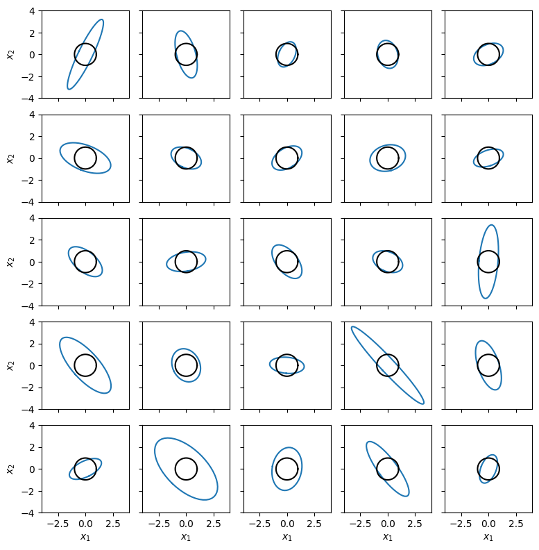
Let $\mbz_1, \ldots, \mbz_{\nu_0}$ be i.i.d. draws from a zero-mean multivariate normal,

\begin{align} \mbz_i \iid{\sim} \cN(\mbzero, \mbLambda_0), \quad i = 1, \ldots, \nu_0. \end{align}

(28)

The sum of outer products $\mbLambda = \sum_{i=1}^{\nu_0} \mbz_i \mbz_i^\top$ is a $D \times D$ random positive semidefinite matrix. It follows a Wishart distribution with $\nu_0$ degrees of freedom and scale $\mbLambda_0$ , written $\mbLambda \sim \mathrm{W}(\nu_0, \mbLambda_0)$ .

Let $\cS_D$ denote the set of $D \times D$ symmetric positive definite matrices. For $\mbLambda \in \cS_D$ , the Wishart pdf is,

\begin{align} \mathrm{W}(\mbLambda \mid \nu_0, \mbLambda_0) &= \frac{1}{2^{\frac{\nu_0 D}{2}}\left|\mbLambda_0\right|^{\frac{\nu_0}{2}}\Gamma_{D}\!\left({\frac{\nu_0}{2}}\right)} {\left| \mbLambda \right|}^{\frac{\nu_0-D-1}{2}} \exp\!\left(-\tfrac{1}{2} \Tr(\mbLambda_0^{-1}\mbLambda)\right), \end{align}

(29)

where $\Gamma_D$ is the multivariate gamma function, defined as

\begin{align} \Gamma_D(a) = \pi^{D(D-1)/4} \prod_{d=1}^D \Gamma\!\left(a + \frac{1-d}{2}\right). \end{align}

(30)

The parameters are: $\nu_0 > D - 1$ degrees of freedom (which must exceed $D-1$ for the distribution to be proper) and $\mbLambda_0 \in \cS_D$ , the scale matrix. The mean and mode are,

\begin{align} \E[\mbLambda] &= \nu_0 \mbLambda_0, \quad \text{and} \quad \mathrm{mode}[\mbLambda] = (\nu_0 - D - 1)\mbLambda_0 \quad \text{for } \nu_0 \geq D+1. \end{align}

(31)

In the univariate case $D=1$ : $\mathrm{W}(\lambda \mid \nu_0, \nu_0^{-1} \lambda_0) = \chi^2(\nu_0, \lambda_0)$ , which confirms the connection to the scaled chi-squared distribution.

The Wishart distribution plays a key role in two different settings. In frequentist statistics, it is the sampling distribution of the precision matrix estimated from multivariate normal data. In Bayesian statistics, it is the conjugate prior for the precision matrix of a multivariate normal, as we will see next.

torch.manual_seed(305)

ν0 = torch.tensor(4.)
Λ0 = torch.eye(2) / ν0
Λs = Wishart(ν0, covariance_matrix=Λ0).sample(sample_shape=(5, 5))

fig, axs = plt.subplots(5, 5, figsize=(8, 8), sharex=True, sharey=True)
for i in range(5):
    for j in range(5):
        plot_cov(torch.inverse(Λs[i, j]), ax=axs[i, j])
        plot_cov(torch.eye(2), ax=axs[i, j], color='k')
        axs[i, j].set_xlim(-4, 4)
        axs[i, j].set_ylim(-4, 4)
        axs[i, j].set_aspect(1)
for i in range(5):
    axs[i, 0].set_ylabel(r"$x_2$")
    axs[-1, i].set_xlabel(r"$x_1$")
plt.tight_layout()

/opt/hostedtoolcache/Python/3.13.13/x64/lib/python3.13/site-packages/torch/distributions/distribution.py:173: UserWarning: Singular sample detected.
  return self.rsample(sample_shape)

Bayesian Estimation: Unknown Precision¶

With the Wishart distribution in hand, we can perform Bayesian inference for an unknown precision matrix:

\begin{align} \mbLambda &\sim \mathrm{W}(\nu_0, \mbLambda_0), \\ \mbx_n &\iid{\sim} \cN(\mbmu, \mbLambda^{-1}). \end{align}

(32)

To compute the posterior $p(\mbLambda \mid \mbX, \mbeta)$ with $\mbeta = (\mbmu, \nu_0, \mbLambda_0)$ , we expand the Wishart prior and the Gaussian likelihood, collecting terms in $\mbLambda$ ,

\begin{align} p(\mbLambda \mid \mbX, \mbeta) &\propto \mathrm{W}(\mbLambda \mid \nu_0, \mbLambda_0) \prod_{n=1}^N \cN(\mbx_n \mid \mbmu, \mbLambda^{-1}) \\ &\propto |\mbLambda|^{\frac{\nu_0 - D - 1}{2}} e^{-\frac{1}{2} \Tr(\mbLambda_0^{-1} \mbLambda)} \cdot \prod_{n=1}^N |\mbLambda|^{\frac{1}{2}} e^{-\frac{1}{2} (\mbx_n - \mbmu)^\top \mbLambda (\mbx_n - \mbmu)} \\ &\propto |\mbLambda|^{\frac{\nu_0 + N - D - 1}{2}} \exp\!\left(-\tfrac{1}{2} \Tr\!\left(\left[\mbLambda_0^{-1} + \sum_{n=1}^N (\mbx_n -\mbmu) (\mbx_n - \mbmu)^\top \right] \mbLambda \right)\right). \end{align}

(33)

In the last step we used the identity $(\mbx_n - \mbmu)^\top \mbLambda (\mbx_n - \mbmu) = \Tr(\mbLambda (\mbx_n - \mbmu)(\mbx_n - \mbmu)^\top)$ to consolidate the exponential. The result has exactly the form of a Wishart density, so the posterior is,

\begin{align} p(\mbLambda \mid \mbX, \mbeta) &= \mathrm{W}(\mbLambda \mid \nu_N, \mbLambda_N), \end{align}

(34)

where

\begin{align} \nu_N &= \nu_0 + N, \\ \mbLambda_N &= \left[\mbLambda_0^{-1} + \sum_{n=1}^N (\mbx_n -\mbmu) (\mbx_n - \mbmu)^\top \right]^{-1}. \end{align}

(35)

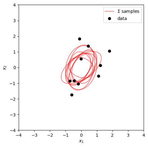
The degrees of freedom simply accumulate: each new observation adds 1 to $\nu_N$ , increasing our certainty about $\mbLambda$ . The posterior scale $\mbLambda_N$ is the inverse of the sum of the prior inverse scale and the data scatter matrix $\sum_n (\mbx_n - \mbmu)(\mbx_n - \mbmu)^\top$ . In the large data limit, the posterior mean $\nu_N \mbLambda_N$ converges to $\bigl(\frac{1}{N}\sum_{n} (\mbx_n - \mbmu)(\mbx_n - \mbmu)^\top\bigr)^{-1}$ , the inverse of the sample covariance — as we would expect.

The Inverse Wishart Distribution¶

When it is more natural to parameterize in terms of the covariance $\mbSigma$ rather than the precision $\mbLambda$ , we use the inverse Wishart distribution. It is defined simply by a change of variables: if $\mbLambda \sim \mathrm{W}(\nu_0, \mbLambda_0)$ , then $\mbSigma = \mbLambda^{-1}$ follows an inverse Wishart distribution,

\begin{align} \mbLambda \sim \mathrm{W}(\nu_0, \mbLambda_0) \iff \mbSigma = \mbLambda^{-1} \sim \mathrm{IW}(\nu_0, \mbSigma_0), \end{align}

(36)

where $\mbSigma_0 = \mbLambda_0^{-1}$ . Its pdf is,

\begin{align} \mathrm{IW}(\mbSigma \mid \nu_0, \mbSigma_0) &= \frac{\left|\mbSigma_0\right|^{\frac{\nu_0}{2}}}{2^{\frac{\nu_0 D}{2}}\Gamma_{D}\!\left({\frac{\nu_0}{2}}\right)} {\left| \mbSigma \right|}^{-\frac{\nu_0+D+1}{2}} \exp\!\left(-\tfrac{1}{2} \Tr(\mbSigma_0 \mbSigma^{-1})\right). \end{align}

(37)

The parameters are the same degrees of freedom $\nu_0$ and a scale matrix $\mbSigma_0 \in \cS_D$ . Its mean and mode are,

\begin{align} \E[\mbSigma] &= \frac{\mbSigma_0}{\nu_0 - D - 1} \quad \text{for } \nu_0 > D+1, \quad \text{and} \quad \mathrm{mode}[\mbSigma] = \frac{\mbSigma_0}{\nu_0 + D + 1}. \end{align}

(38)

The scale matrix $\mbSigma_0$ can be interpreted as a prior sum of squared deviations, and $\nu_0$ controls how tightly concentrated the prior is around $\frac{\mbSigma_0}{\nu_0 - D - 1}$ . In the univariate case $D=1$ : $\mathrm{IW}(\sigma^2 \mid \nu_0, \nu_0 \sigma_0^2) = \chi^{-2}(\nu_0, \sigma_0^2)$ , recovering the scaled inverse chi-squared from Lecture 1.

Exercise

Consider the model with unknown covariance,

\begin{align} \mbSigma &\sim \mathrm{IW}(\nu_0, \mbSigma_0), \\ \mbx_n &\iid{\sim} \cN(\mbmu, \mbSigma). \end{align}

(39)

Show that the posterior is also inverse Wishart,

\begin{align} p(\mbSigma \mid \mbX, \mbeta) &= \mathrm{IW}(\nu_N, \mbSigma_N), \end{align}

(40)

where

\begin{align} \nu_N &= \nu_0 + N, \\ \mbSigma_N &= \mbSigma_0 + \sum_{n=1}^N (\mbx_n - \mbmu) (\mbx_n - \mbmu)^\top. \end{align}

(41)

Interpret the update: $\mbSigma_N$ is the prior scale matrix plus the empirical scatter matrix.

torch.manual_seed(305)

N  = 10
X  = MultivariateNormal(torch.zeros(2), torch.eye(2)).sample((N,))

ν0 = torch.tensor(1.0)
Λ0 = torch.eye(2)
νN = ν0 + N
ΛN = torch.inverse(torch.inverse(Λ0) + X.T @ X)

Λ_samp = Wishart(νN, ΛN).sample((10,))
Σ_samp = torch.inverse(Λ_samp)

fig, ax = plt.subplots()
ax.set_aspect(1)
for i, Σ in enumerate(Σ_samp):
    plot_cov(Σ, ax=ax, color='r', alpha=0.5,
             label=r"$\Sigma$ samples" if i == 0 else None)
ax.plot(X[:, 0], X[:, 1], 'ko', markersize=6, label="data")
ax.set_xlim(-4, 4)
ax.set_ylim(-4, 4)
ax.set_xlabel(r"$x_1$")
ax.set_ylabel(r"$x_2$")
ax.legend()
plt.tight_layout()

Normal-Inverse-Wishart Prior¶

In the most general setting, both $\mbmu$ and $\mbSigma$ are unknown. Following the same strategy as Lecture 1 for the univariate case, we construct a joint conjugate prior over $(\mbmu, \mbSigma)$ . The key idea is to express the joint prior as a product $p(\mbmu, \mbSigma) = p(\mbmu \mid \mbSigma) \, p(\mbSigma)$ , choosing each factor to be conjugate in a compatible way.

Specifically, we set the prior on the covariance to be inverse Wishart and — crucially — make the prior on the mean conditional on the covariance: $\mbmu \mid \mbSigma \sim \cN(\mbmu_0, \mbSigma / \kappa_0)$ . This coupling between the mean and covariance priors, where the uncertainty in $\mbmu$ scales with $\mbSigma / \kappa_0$ , is what makes the joint prior conjugate. The result is the normal-inverse-Wishart (NIW) distribution,

\begin{align} \mathrm{NIW}(\mbmu, \mbSigma \mid \mbmu_0, \kappa_0, \nu_0, \mbSigma_0) &= \cN(\mbmu \mid \mbmu_0, \mbSigma / \kappa_0) \, \mathrm{IW}(\mbSigma \mid \nu_0, \mbSigma_0). \end{align}

(42)

The four hyperparameters have natural interpretations: $\mbmu_0$ is the prior mean, $\kappa_0$ is the mean confidence (how many pseudo-observations worth of information we have about the mean), $\nu_0$ is the degrees of freedom for the covariance, and $\mbSigma_0$ is the prior scale for the covariance.

Exercise

Consider the model $(\mbmu, \mbSigma) \sim \mathrm{NIW}(\mbmu_0, \kappa_0, \nu_0, \mbSigma_0)$ and $\mbx_n \iid{\sim} \cN(\mbmu, \mbSigma)$ . Show that the posterior is,

\begin{align} p(\mbmu, \mbSigma \mid \mbX) &= \mathrm{NIW}(\mbmu_N, \kappa_N, \nu_N, \mbSigma_N), \end{align}

(43)

where

\begin{align} \kappa_N &= \kappa_0 + N, \\ \nu_N &= \nu_0 + N, \\ \mbmu_N &= \frac{\kappa_0 \mbmu_0 + \sum_{n=1}^N \mbx_n}{\kappa_N} = \frac{\kappa_0}{\kappa_N} \mbmu_0 + \frac{N}{\kappa_N} \bar{\mbx}, \\ \mbSigma_N &= \mbSigma_0 + \kappa_0 \mbmu_0\mbmu_0^\top + \sum_{n=1}^N \mbx_n \mbx_n^\top - \kappa_N \mbmu_N \mbmu_N^\top. \end{align}

(44)

Notice that $\mbmu_N$ is a weighted average of the prior mean $\mbmu_0$ and the sample mean $\bar{\mbx}$ , with weights $\kappa_0 / \kappa_N$ and $N / \kappa_N$ respectively.

Posterior Marginals¶

Just as in the univariate case (where the marginal of the mean under a normal-inverse-chi-squared posterior was a Student’s t distribution), the posterior marginal of $\mbmu$ under the NIW is a multivariate Student’s t.

Integrating out $\mbSigma$ ,

\begin{align} p(\mbmu \mid \mbX) &= \int p(\mbmu, \mbSigma \mid \mbX) \dif \mbSigma \\ &= \int \cN(\mbmu \mid \mbmu_N, \mbSigma / \kappa_N) \, \mathrm{IW}(\mbSigma \mid \nu_N, \mbSigma_N) \dif \mbSigma \\ &= \mathrm{St}\!\left(\nu_N - D + 1,\; \mbmu_N,\; \frac{\mbSigma_N}{\kappa_N (\nu_N - D + 1)} \right). \end{align}

(45)

The Student’s t distribution arises because we are averaging a Gaussian over a random covariance drawn from an inverse Wishart — the extra uncertainty about $\mbSigma$ inflates the tails of the marginal compared to a pure Gaussian. The multivariate Student’s t distribution with $\nu$ degrees of freedom, location $\mbmu$ , and scale matrix $\mbSigma$ has density,

\begin{align} \mathrm{St}(\mbx \mid \nu, \mbmu, \mbSigma) &= \frac{\Gamma\!\left(\frac{\nu + D}{2}\right)}{\Gamma\!\left(\frac{\nu}{2}\right)} (\nu \pi)^{-\frac{D}{2}} |\mbSigma|^{-\frac{1}{2}} \left[1 + \frac{\Delta^2}{\nu} \right]^{-\frac{\nu + D}{2}}, \end{align}

(46)

where $\Delta^2 = (\mbx - \mbmu)^\top \mbSigma^{-1} (\mbx - \mbmu)$ is the squared Mahalanobis distance. When $\nu$ is large, the term $[1 + \Delta^2/\nu]^{-(\nu+D)/2}$ converges to $e^{-\Delta^2/2}$ and the Student’s t approaches a Gaussian. When $\nu$ is small, the distribution has heavier tails than a Gaussian. The mean of the multivariate Student’s t is $\mbmu$ and the covariance is $\frac{\nu}{\nu - 2} \mbSigma$ (for $\nu > 2$ ) — the extra factor of $\nu / (\nu - 2) > 1$ reflects the heavier tails.

In our posterior, the effective degrees of freedom $\nu_N - D + 1 = \nu_0 + N - D + 1$ grow with the number of observations, so the posterior predictive distribution converges to a Gaussian as $N \to \infty$ , as we would expect when we become certain about $\mbSigma$ .

Conclusion¶

The multivariate normal distribution is the cornerstone of high-dimensional probabilistic modeling. Its key analytical properties — the ability to marginalize and condition in closed form, the Schur complement formula for conditional means and variances, and the Woodbury identity for efficient precision-form updates — appear repeatedly throughout the course. The conjugate prior framework generalizes naturally from the scalar case: the Wishart and inverse-Wishart distributions are the natural conjugates for the precision and covariance respectively, and the normal-inverse-Wishart prior gives a joint conjugate for unknown mean and covariance. The posterior marginal of the mean is a multivariate Student’s t, reflecting additional uncertainty from integrating out the unknown covariance.

References

1. Bishop, C. M. (2006). Pattern recognition and machine learning. Springer.
2. Murphy, K. P. (2023). Probabilistic Machine Learning: Advanced Topics. MIT Press. https://probml.github.io/pml-book/book2.html