Probabilistic Graphical Models

Directed graphical models (DGMs) provide a language for representing joint distributions over many variables compactly. By encoding conditional independence assumptions as a directed acyclic graph (DAG), we can specify and reason about high-dimensional distributions that would otherwise be intractable.

In this lecture we cover:

Product-rule factorization and the DAG representation
Plate notation for repeated structure
Conditional independence and the Markov blanket
Exchangeability and de Finetti’s theorem

import io
import matplotlib.pyplot as plt
import matplotlib.image as mpimg
from daft import PGM

def pgm_to_img(pgm):
    """Render a PGM to an RGBA image array."""
    pgm.render()
    ax = plt.gca()
    ax.set_aspect('equal')
    buf = io.BytesIO()
    fig = plt.gcf()
    fig.savefig(buf, format='png', bbox_inches='tight', dpi=150)
    buf.seek(0)
    img = mpimg.imread(buf)
    plt.close(fig)
    return img

Directed Graphical Models¶

Motivation¶

Consider a joint distribution $p(x_1, \ldots, x_D)$ over $D$ discrete variables, each taking values in $\{1, \ldots, K\}$ . An arbitrary distribution on $D$ such variables requires $K^D - 1$ parameters — exponential in $D$ . Even for modest $D$ and $K$ this is enormous.

The product rule always lets us factor any joint distribution as a chain,

\begin{align} p(\mbx) &= p(x_1) \, p(x_2 \mid x_1) \, p(x_3 \mid x_1, x_2) \cdots p(x_D \mid x_1, \ldots, x_{D-1}). \end{align}

(1)

But this representation is equally expensive: conditioning on all preceding variables.

The key idea of graphical models is that many conditional independencies in real-world distributions make most of these conditions unnecessary. If $x_d$ only depends on a small subset $\mathsf{pa}_d \subseteq \{1, \ldots, d-1\}$ of the preceding variables (its parents), then

\begin{align} p(\mbx) &= \prod_{d=1}^D p(x_d \mid \mbx_{\mathsf{pa}_d}). \end{align}

(2)

The number of parameters is now $\sum_{d=1}^D K^{|\mathsf{pa}_d|}$ , which is manageable when $|\mathsf{pa}_d|$ is small.

Definition¶

A directed graphical model (DGM), or Bayesian network, represents this factorization as a directed acyclic graph (DAG):

Each node corresponds to a variable $x_d$ — it may be discrete or continuous, scalar or multidimensional.
A directed edge from node $i$ to node $j$ means $i \in \mathsf{pa}_j$ .
The graph must be acyclic (no directed cycles), which ensures the product factorization is well-defined.

The absence of an edge from $i$ to $j$ encodes a conditional independence assumption: $x_j$ does not depend directly on $x_i$ (given $x_j$ ’s other parents). The more edges we omit, the more compact the representation.

# DAG for p(x1)p(x2)p(x3)p(x4|x1,x2,x3)p(x5|x1,x3)p(x6|x4)p(x7|x4,x5)
pgm = PGM()

# Row 0 (top): roots x1, x2, x3
pgm.add_node("x1", r"$x_1$", 0, 2)
pgm.add_node("x2", r"$x_2$", 2, 2)
pgm.add_node("x3", r"$x_3$", 4, 2)

# Row 1: x4, x5
pgm.add_node("x4", r"$x_4$", 1, 1)
pgm.add_node("x5", r"$x_5$", 3, 1)

# Row 2 (bottom): x6, x7
pgm.add_node("x6", r"$x_6$", 0, 0)
pgm.add_node("x7", r"$x_7$", 2, 0)

# Edges
for u, v in [("x1","x4"),("x2","x4"),("x3","x4"),
             ("x1","x5"),("x3","x5"),
             ("x4","x6"),("x4","x7"),("x5","x7")]:
    pgm.add_edge(u, v)

pgm.render()
plt.gca().set_aspect('equal')
plt.show()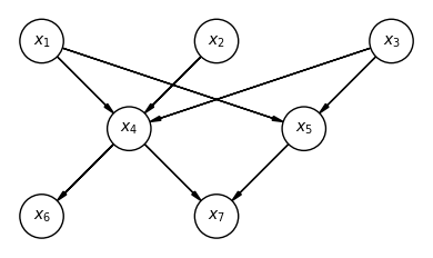

<Figure size 370.079x212.598 with 1 Axes>

Plate Notation¶

Many probabilistic models have repeated structure — the same conditional distribution applied to many variables. For example, the diagonal-covariance Gaussian,

\begin{align} \cN(\mbx \mid \mbmu, \sigma^2 \mbI) &= \prod_{d=1}^D \cN(x_d \mid \mu_d, \sigma^2), \end{align}

(4)

describes $D$ independent variables sharing the same conditional form. Drawing $D$ separate nodes would be redundant.

Plate notation compresses repeated structure by drawing a single representative node inside a rectangle (the plate), labelled with the index set. A node outside the plate is shared across all repetitions; a node inside is replicated once per index.

Plates can be nested: a plate labelled $n = 1, \ldots, N$ inside a plate labelled $s = 1, \ldots, S$ represents $N \times S$ variables, one for each $(n, s)$ pair. We will use nested plates extensively in the hierarchical model below.

The figure below shows how a shared parameter $\theta$ generating $N$ i.i.d. observations $x_n$ is written in plate notation. Shaded nodes denote observed variables.

# Plate notation: shared theta, N i.i.d. observed x_n
pgm = PGM()
pgm.add_node("theta", r"$\theta$", 1, 2)
pgm.add_node("xn", r"$x_n$", 1, 1, observed=True)
pgm.add_plate([0.4, 0.4, 1.2, 1.2], label=r"$n = 1, \ldots, N$",
              position="bottom right")
pgm.add_edge("theta", "xn")

pgm.render()
plt.gca().set_aspect('equal')
plt.show()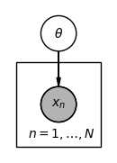

<Figure size 110.236x161.417 with 1 Axes>

Conditional Independence¶

We write $x_i \perp\!\!\!\perp x_j \mid \mbx_s$ if $x_i$ and $x_j$ are conditionally independent given $\mbx_s$ :

\begin{align} p(x_i \mid x_j, \mbx_s) &= p(x_i \mid \mbx_s). \end{align}

(5)

Conditional independencies in a DGM can be read off by examining three basic motifs (see Murphy or Bishop for the full d-separation rules):

Chain $x_i \to x_k \to x_j$ : $x_i \perp\!\!\!\perp x_j \mid x_k$ (conditioning on the middle node blocks the path).
Fork $x_i \leftarrow x_k \to x_j$ : $x_i \perp\!\!\!\perp x_j \mid x_k$ (conditioning on the common cause blocks the path).
Collider $x_i \to x_k \leftarrow x_j$ : $x_i \not\perp\!\!\!\perp x_j \mid x_k$ (conditioning on a common effect opens a previously blocked path — often called explaining away).

# Three d-separation motifs: chain, fork, collider
fig, axes = plt.subplots(1, 3, figsize=(9, 2.5))

for ax, (title, edges) in zip(axes, [
    ("Chain",    [("xi","xk"),("xk","xj")]),
    ("Fork",     [("xk","xi"),("xk","xj")]),
    ("Collider", [("xi","xk"),("xj","xk")]),
]):
    pgm = PGM()
    pgm.add_node("xi", r"$x_i$", 0, 0)
    pgm.add_node("xk", r"$x_k$", 1, 0)
    pgm.add_node("xj", r"$x_j$", 2, 0)
    for u, v in edges:
        pgm.add_edge(u, v)
    img = pgm_to_img(pgm)
    ax.imshow(img)
    ax.axis("off")
    ax.set_title(title, fontsize=11)

plt.tight_layout()
plt.show()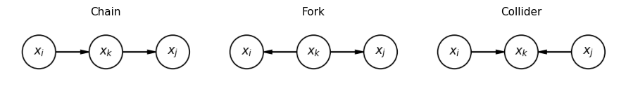

Markov Blanket¶

The Markov blanket of a node $x_d$ is the set of variables that, when conditioned on, render $x_d$ independent of all other variables. In a DGM, the Markov blanket of $x_d$ consists of:

$x_d$ ’s parents,
$x_d$ ’s children, and
the other parents of $x_d$ ’s children (the co-parents).

These are exactly the variables that appear alongside $x_d$ in at least one factor of the joint distribution. Given its Markov blanket, $x_d$ is conditionally independent of all remaining variables — a fact we will exploit repeatedly in deriving conditional posteriors.

Exchangeability and de Finetti’s Theorem¶

Suppose we want to model a collection of variables $(x_1, \ldots, x_N)$ and have no information that distinguishes or orders them. A natural requirement is exchangeability: the joint distribution is invariant to any permutation $\pi$ ,

\begin{align} p(x_1, \ldots, x_N) &= p(x_{\pi(1)}, \ldots, x_{\pi(N)}). \end{align}

(6)

The simplest exchangeable distribution assumes the variables are i.i.d., $p(\mbx) = \prod_n p(x_n)$ . More generally, we may assume the variables are conditionally independent given a latent parameter $\theta$ which is marginalized over,

\begin{align} p(x_1, \ldots, x_N) &= \int \left[\prod_{n=1}^N p(x_n \mid \theta)\right] p(\theta) \dif \theta. \end{align}

(7)

Marginally, the $x_n$ are not independent — observing some $x_n$ updates our belief about $\theta$ and therefore about other $x_{n'}$ . But they are exchangeable.

De Finetti’s theorem states that as $N \to \infty$ , any suitably well-behaved exchangeable distribution on $(x_1, \ldots, x_N)$ can be represented in exactly this mixture form. The theorem does not hold in general for finite $N$ , but it provides a compelling motivation for Bayesian hierarchical models: placing a prior over $\theta$ and conditioning on the data is the correct procedure when observations are exchangeable.

Conclusion¶

Directed graphical models provide a principled way to represent the conditional independence structure of a joint distribution. The key results are:

Any joint distribution factors as a product of conditionals over a DAG; absent edges encode conditional independence assumptions that reduce the number of parameters.
Plate notation compresses repeated structure and makes hierarchical models easy to read.
The Markov blanket of a node determines its complete conditional — the ingredient needed for Gibbs sampling (Lecture 5).
Exchangeability motivates placing a shared prior over group-level parameters, and de Finetti’s theorem gives this practice a theoretical foundation.