Hierarchical Gaussian Models

This lecture works through exact Bayesian inference in a hierarchical Gaussian model — a multi-level model that pools information across groups. The running example is the Eight Schools dataset from Gelman et al., 2013, used as a benchmark by many probabilistic programming systems.

The model places a shared prior over school-level means, allowing estimates to borrow strength from one another while still respecting per-school data. Because the model is conditionally linear and Gaussian, the posterior can be computed exactly by sequential marginalization — making this one of the most complex models for which closed-form inference is still achievable.

In this lecture we cover:

The hierarchical Gaussian model and its graphical representation
Sequential marginalization: $p(\mbtheta \mid \cdot)$ , $p(\mu \mid \tau^2, \cdot)$ , $p(\tau^2 \mid \cdot)$
Numerical normalization of the one-dimensional marginal $p(\tau^2 \mid \mbX)$
Posterior sampling via ancestral sampling
Comparison to classical ANOVA / partial pooling

import torch
from torch.distributions import Normal, Gamma, Categorical, TransformedDistribution
from torch.distributions.transforms import PowerTransform
import matplotlib.pyplot as plt
from matplotlib.cm import Blues


class ScaledInvChiSq(TransformedDistribution):
    """Scaled inverse chi-squared: χ⁻²(ν, σ²).

    Equivalent to IGa(ν/2, νσ²/2). Implemented as a transformation of Gamma.
    """
    def __init__(self, ν, σ2):
        base = Gamma(ν / 2, ν * σ2 / 2)
        TransformedDistribution.__init__(self, base, [PowerTransform(-1)])
        self.ν  = ν
        self.σ2 = σ2

Motivation¶

Data are often organized into groups — students within schools, patients within hospitals, experiments within labs. The individual observations within a group are not exchangeable with those in other groups (because group membership matters), but the groups themselves may be exchangeable.

Hierarchical models handle this by introducing group-level parameters $\theta_s$ (one per group $s$ ), drawn i.i.d. from a shared population distribution. Group-level parameters explain within-group variation, while the population distribution allows information to be shared across groups.

The key insight is that the scores within each school are not exchangeable with those across schools, but the schools themselves are exchangeable. This motivates the following hierarchical model:

\begin{align} \mu, \tau^2 &\sim p(\mu, \tau^2), \\ \theta_s \mid \mu, \tau^2 &\iid{\sim} \cN(\mu, \tau^2), \quad s = 1, \ldots, S, \\ x_{s,n} \mid \theta_s &\iid{\sim} \cN(\theta_s, \sigma_s^2), \quad n = 1, \ldots, N_s. \end{align}

(1)

Each school has its own mean $\theta_s$ , drawn from a global distribution with mean $\mu$ and variance $\tau^2$ . The global mean $\mu$ captures the overall population effect; the global variance $\tau^2$ controls how much schools differ from each other.

For the prior on $(\mu, \tau^2)$ , we use a normal-inverse-chi-squared distribution (as in Lecture 2 but for the scalar case):

\begin{align} p(\mu, \tau^2) &= \mathrm{NIX}(\mu, \tau^2 \mid \mu_0, \kappa_0, \nu_0, \tau_0^2) = \cN(\mu \mid \mu_0, \tau^2 / \kappa_0) \, \chi^{-2}(\tau^2 \mid \nu_0, \tau_0^2). \end{align}

(2)

The hyperparameters are $\boldsymbol{\eta} = (\mu_0, \kappa_0, \nu_0, \tau_0^2, \{\sigma_s^2\}_{s=1}^S)$ .

The Eight Schools Dataset¶

We illustrate with a classic dataset from Gelman et al., 2013, Ch 5.5, also used as a benchmark by probabilistic programming systems such as Stan and NumPyro. Eight schools participated in a study of an SAT coaching program. For each school $s$ , we are given the estimated treatment effect $\bar{x}_s$ (the difference in mean SAT scores between coached and uncoached students) and its standard error $\bar{\sigma}_s$ .

School	$\bar{x}_s$	$\bar{\sigma}_s$
A	28	15
B	8	10
C	−3	16
D	7	11
E	−1	9
F	1	11
G	18	10
H	12	18

The standard errors $\bar{\sigma}_s$ are treated as known (they are themselves estimates from each school’s data, but we condition on them for simplicity). We set weakly informative hyperparameters: $\mu_0 = 0$ , $\kappa_0 = 0.1$ , $\nu_0 = 0.1$ , and $\tau_0^2 = 100$ .

torch.manual_seed(305)

S = 8                        # number of schools

# Hyperparameters
μ0   = torch.tensor(0.0)     # prior mean of global effect
κ0   = torch.tensor(0.1)     # prior concentration (NIX)
ν0   = torch.tensor(0.1)     # degrees of freedom (NIX)
τ2_0 = torch.tensor(100.0)   # prior scale of global variance

# Observed school-level sample means and standard errors
x_bars  = torch.tensor([28., 8., -3., 7., -1., 1., 18., 12.])
σ_bars  = torch.tensor([15., 10., 16., 11., 9., 11., 10., 18.])

Bayesian Inference in the Hierarchical Gaussian Model¶

Our goal is to compute the joint posterior,

\begin{align} p(\mu, \tau^2, \mbtheta \mid \mbX, \boldsymbol{\eta}), \end{align}

(3)

where $\mbtheta = (\theta_1, \ldots, \theta_S)$ . We proceed by sequential marginalization, decomposing the posterior using the product rule:

\begin{align} p(\mu, \tau^2, \mbtheta \mid \mbX, \boldsymbol{\eta}) &= p(\mbtheta \mid \mu, \tau^2, \mbX, \boldsymbol{\eta}) \; p(\mu \mid \tau^2, \mbX, \boldsymbol{\eta}) \; p(\tau^2 \mid \mbX, \boldsymbol{\eta}). \end{align}

(4)

We will compute each factor in turn.

Step 1: Sufficient Statistics¶

As a function of $\theta_s$ , the likelihood for school $s$ depends on the data only through the school mean $\bar{x}_s = \frac{1}{N_s}\sum_n x_{s,n}$ :

\begin{align} \prod_{n=1}^{N_s} \cN(x_{s,n} \mid \theta_s, \sigma_s^2) &\propto \cN(\bar{x}_s \mid \theta_s, \bar{\sigma}_s^2), \end{align}

(5)

where $\bar{\sigma}_s^2 = \sigma_s^2 / N_s$ is the variance of the school mean. The school mean is thus a sufficient statistic for $\theta_s$ . In the Eight Schools dataset, $\bar{x}_s$ and $\bar{\sigma}_s$ are given directly.

Step 2: Per-School Posteriors (given $\mu$ and $\tau^2$ )¶

The per-school parameters $\theta_s$ are conditionally independent given $(\mu, \tau^2)$ , so the posterior factors:

\begin{align} p(\mbtheta \mid \mu, \tau^2, \mbX, \boldsymbol{\eta}) &= \prod_{s=1}^S p(\theta_s \mid \mu, \tau^2, \bar{x}_s). \end{align}

(6)

Each factor is a product of a Gaussian prior and a Gaussian likelihood, so by the results of Lecture 1,

\begin{align} p(\theta_s \mid \mu, \tau^2, \bar{x}_s) &= \cN(\theta_s \mid \hat{\theta}_s, v_s), \end{align}

(7)

where

\begin{align} v_s &= \left(\frac{1}{\bar{\sigma}_s^2} + \frac{1}{\tau^2}\right)^{-1}, \qquad \hat{\theta}_s = v_s \left(\frac{\bar{x}_s}{\bar{\sigma}_s^2} + \frac{\mu}{\tau^2}\right). \end{align}

(8)

The conditional posterior mean $\hat{\theta}_s$ is a precision-weighted average of the school observation $\bar{x}_s$ and the global mean $\mu$ . When $\tau^2$ is large (schools vary a lot), the school mean dominates; when $\tau^2$ is small, the global mean dominates — this is the shrinkage or partial pooling effect.

Step 3: Posterior of the Global Mean (given $\tau^2$ )¶

To find $p(\mu \mid \tau^2, \mbX, \boldsymbol{\eta})$ , we integrate over $\mbtheta$ . Because each $\theta_s$ enters the model linearly, the integral is tractable via the linear Gaussian model results from Lecture 2:

\begin{align} p(\mu \mid \tau^2, \mbX, \boldsymbol{\eta}) &\propto \cN(\mu \mid \mu_0, \tau^2/\kappa_0) \prod_{s=1}^S \int \cN(\theta_s \mid \mu, \tau^2)\, \cN(\bar{x}_s \mid \theta_s, \bar{\sigma}_s^2)\, \dif\theta_s \\ &= \cN(\mu \mid \mu_0, \tau^2/\kappa_0) \prod_{s=1}^S \cN(\bar{x}_s \mid \mu, \bar{\sigma}_s^2 + \tau^2). \end{align}

(9)

Each integral collapses $\theta_s$ by the linear Gaussian marginalization formula: $\bar{x}_s \mid \mu \sim \cN(\mu, \bar{\sigma}_s^2 + \tau^2)$ .

Collecting terms quadratic and linear in $\mu$ and completing the square gives,

\begin{align} p(\mu \mid \tau^2, \mbX, \boldsymbol{\eta}) &= \cN(\mu \mid \hat{\mu}, v_\mu), \end{align}

(10)

where

\begin{align} \lambda_0 &= \kappa_0 / \tau^2, \quad \lambda_s = 1 / (\bar{\sigma}_s^2 + \tau^2), \\ v_\mu &= \frac{1}{\lambda_0 + \sum_s \lambda_s}, \quad \hat{\mu} = v_\mu \!\left(\lambda_0 \mu_0 + \sum_s \lambda_s \bar{x}_s\right). \end{align}

(11)

The posterior mean $\hat{\mu}$ is a precision-weighted average of the prior mean $\mu_0$ and the school means $\bar{x}_s$ . Schools with smaller total variance $\bar{\sigma}_s^2 + \tau^2$ (i.e. more precisely measured and more similar to the global mean) receive more weight.

def compute_posterior_mu(τ2, μ0, κ0, x_bars, σ_bars):
    """Posterior mean and variance of μ given τ² and data.

    Returns (μ_hat, v_μ), each of shape (T,) for a length-T tensor of τ² values.
    """
    λ0    = κ0 / τ2                                         # (T,)
    λs    = 1 / (σ_bars[None, :]**2 + τ2[:, None])         # (T, S)
    v_μ   = 1 / (λ0 + λs.sum(-1))                          # (T,)
    μ_hat = v_μ * (λ0 * μ0 + (λs * x_bars[None, :]).sum(-1))
    return μ_hat, v_μ

τ2s = torch.tensor([1., 4., 9., 16., 25.])
μ_hat, v_μ = compute_posterior_mu(τ2s, μ0, κ0, x_bars, σ_bars)

μ_grid = torch.linspace(-10, 30, 200)
fig, ax = plt.subplots()
for τ2, mean, var in zip(τ2s, μ_hat, v_μ):
    ax.plot(μ_grid,
            torch.exp(Normal(mean, torch.sqrt(var)).log_prob(μ_grid)),
            color=Blues((τ2 / τ2s.max()).item()),
            label=r"$\tau^2 = {:.0f}$".format(τ2))
ax.set_xlabel(r"$\mu$")
ax.set_ylabel(r"$p(\mu \mid \tau^2, \mathbf{X}, {\eta})$")
ax.legend()
plt.tight_layout()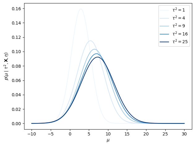

Step 4: Marginal Posterior of $\tau^2$ ¶

The last and hardest term is the marginal posterior of $\tau^2$ , obtained by integrating out $\mu$ :

\begin{align} p(\tau^2 \mid \mbX, \boldsymbol{\eta}) &\propto \int p(\mu, \tau^2, \mbX \mid \boldsymbol{\eta})\, \dif\mu. \end{align}

(12)

Rather than evaluating this integral directly, we use a trick: by Bayes’ rule,

\begin{align} p(\tau^2 \mid \mbX, \boldsymbol{\eta}) &= \frac{p(\mu, \tau^2 \mid \mbX, \boldsymbol{\eta})}{p(\mu \mid \tau^2, \mbX, \boldsymbol{\eta})}, \end{align}

(13)

which holds for any choice of $\mu$ . Substituting the known expressions and evaluating at $\mu = \hat{\mu}$ (which cancels the denominator’s exponential term), we obtain an unnormalized function,

\begin{align} f(\tau^2) \triangleq p(\tau^2) \cdot \frac{\sqrt{v_\mu}}{\tau} \cdot e^{-\frac{\kappa_0}{2\tau^2}(\hat{\mu} - \mu_0)^2} \cdot \prod_{s=1}^S \frac{1}{\sqrt{\bar{\sigma}_s^2 + \tau^2}} \exp\!\left(-\frac{(\bar{x}_s - \hat{\mu})^2}{2(\bar{\sigma}_s^2 + \tau^2)}\right), \end{align}

(14)

where both $\hat{\mu}$ and $v_\mu$ depend on $\tau^2$ . This function has no closed form, but since $\tau^2$ is one-dimensional we can evaluate it on a dense grid and normalize numerically.

def compute_log_f(τ2, x_bars, σ_bars, μ0, κ0, ν0, τ2_0):
    """Compute log f(τ²) — the unnormalized log marginal posterior of τ².

    Args:
        τ2:     (T,) tensor of τ² grid values
        x_bars: (S,) observed school means
        σ_bars: (S,) school standard errors
        μ0, κ0, ν0, τ2_0: NIX hyperparameters

    Returns:
        (T,) tensor of log f(τ²) values
    """
    # Prior on τ²
    log_f = ScaledInvChiSq(ν0, τ2_0).log_prob(τ2)

    # Posterior on μ | τ²  (derived in Step 3)
    λ0    = κ0 / τ2
    λs    = 1 / (σ_bars[None, :]**2 + τ2[:, None])         # (T, S)
    v_μ   = 1 / (λ0 + λs.sum(-1))
    μ_hat = v_μ * (λ0 * μ0 + (λs * x_bars[None, :]).sum(-1))

    # Bayes-rule trick: evaluate at μ = μ_hat
    log_f += 0.5 * torch.log(v_μ) - 0.5 * torch.log(τ2)
    log_f += -0.5 * κ0 / τ2 * (μ_hat - μ0)**2
    log_f += 0.5 * torch.log(λs).sum(-1)
    log_f += -0.5 * (λs * (x_bars[None, :] - μ_hat[:, None])**2).sum(-1)

    return log_f

τ2_grid = torch.linspace(1e-1, 256, 1000)

log_f   = compute_log_f(τ2_grid, x_bars, σ_bars, μ0, κ0, ν0, τ2_0)
dτ2     = τ2_grid[1] - τ2_grid[0]
p_τ2    = torch.exp(log_f - torch.logsumexp(log_f, 0) - torch.log(dτ2))

# Change of variables to get p(τ)
τ_grid  = torch.sqrt(τ2_grid)
p_τ     = 2 * p_τ2 * τ_grid

τ_mean  = (p_τ[:-1] * torch.diff(τ_grid) * τ_grid[:-1]).sum()
τ_var   = (p_τ[:-1] * torch.diff(τ_grid) * (τ_grid[:-1] - τ_mean)**2).sum()
print(f"Posterior  E[τ] = {τ_mean:.2f},  Std[τ] = {τ_var.sqrt():.2f}")

Posterior  E[τ] = 4.46,  Std[τ] = 2.54

fig, axes = plt.subplots(1, 2, figsize=(10, 3))
axes[0].plot(τ2_grid, p_τ2)
axes[0].set_xlabel(r"$\tau^2$")
axes[0].set_ylabel(r"$p(\tau^2 \mid \mathbf{X}, {\eta})$")
axes[0].set_ylim(0)
axes[0].grid(True)

axes[1].plot(τ_grid, p_τ)
axes[1].set_xlabel(r"$\tau$")
axes[1].set_ylabel(r"$p(\tau \mid \mathbf{X}, {\eta})$")
axes[1].set_ylim(0)
axes[1].grid(True)

plt.tight_layout()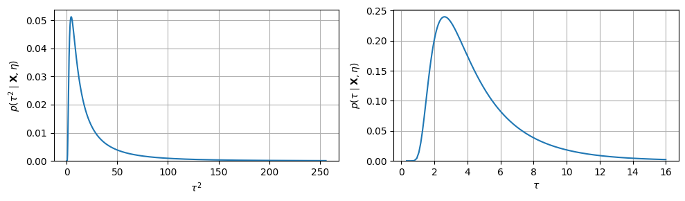

Step 5: Per-School Effects Marginalizing over $\mu$ ¶

Finally, we want the marginal posterior of each $\theta_s$ given $\tau^2$ and the data, having integrated out $\mu$ . Using the product rule,

\begin{align} p(\theta_s \mid \tau^2, \mbX, \boldsymbol{\eta}) &= \int p(\theta_s \mid \mu, \tau^2, \bar{x}_s) \, p(\mu \mid \tau^2, \mbX, \boldsymbol{\eta}) \, \dif\mu. \end{align}

(15)

Both factors are Gaussian in $\mu$ , so the integral is again tractable via linear Gaussian marginalization:

\begin{align} p(\theta_s \mid \tau^2, \mbX, \boldsymbol{\eta}) &= \cN(\theta_s \mid \hat{\theta}_s, v_{\theta_s}), \end{align}

(16)

where

\begin{align} v_{\theta_s} &= \left(\frac{1}{\bar{\sigma}_s^2} + \frac{1}{\tau^2 + v_\mu}\right)^{-1}, \qquad \hat{\theta}_s = v_{\theta_s}\left(\frac{\bar{x}_s}{\bar{\sigma}_s^2} + \frac{\hat{\mu}}{\tau^2 + v_\mu}\right). \end{align}

(17)

The additional $v_\mu$ term in the denominator inflates the effective variance of the prior on $\theta_s$ , reflecting our residual uncertainty about $\mu$ .

def compute_posterior_theta(τ2, μ, x_bars, σ_bars):
    """Posterior mean/variance of θ_s given τ², μ, and data.

    Broadcasts over (T,) tensors of τ² and μ.
    Returns (θ_hat, v_θ) each of shape (T, S).
    """
    v_θ   = 1 / (1/σ_bars[None,:]**2 + 1/τ2[:,None])
    θ_hat = v_θ * (x_bars[None,:]/σ_bars[None,:]**2 + μ[:,None]/τ2[:,None])
    return θ_hat, v_θ


def compute_posterior_theta_marg(τ2, μ0, κ0, x_bars, σ_bars):
    """Posterior mean/variance of θ_s given τ², marginalizing over μ.

    Returns (θ_hat, v_θ) each of shape (T, S).
    """
    μ_hat, v_μ = compute_posterior_mu(τ2, μ0, κ0, x_bars, σ_bars)
    v_θ   = 1 / (1/σ_bars[None,:]**2 + 1/(τ2[:,None] + v_μ[:,None]))
    θ_hat = v_θ * (x_bars[None,:]/σ_bars[None,:]**2
                   + μ_hat[:,None]/(τ2[:,None] + v_μ[:,None]))
    return θ_hat, v_θ

θ_hat, v_θ = compute_posterior_theta_marg(τ2_grid, μ0, κ0, x_bars, σ_bars)

fig, ax = plt.subplots()
for s in range(S):
    ax.plot(τ_grid, θ_hat[:, s], label=f"School {s+1}")
ax.set_xlabel(r"$\tau$")
ax.set_ylabel(r"$\mathbb{E}[\theta_s \mid \tau, \mathbf{X}, {\eta}]$")
ax.legend(fontsize=8, ncol=2)
plt.tight_layout()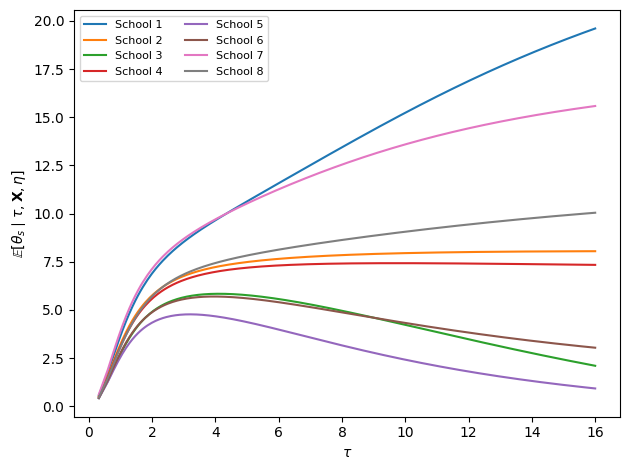

Posterior Sampling via Ancestral Sampling¶

We now have all the pieces needed to draw samples from the joint posterior $p(\mu, \tau^2, \mbtheta \mid \mbX, \boldsymbol{\eta})$ . Because we computed the posterior in the order $\tau^2 \to \mu \to \mbtheta$ (by sequential marginalization), we can draw samples in the reverse order — this is called ancestral sampling:

Sample $\tau$ from the normalized grid approximation $p(\tau \mid \mbX, \boldsymbol{\eta})$ .
Sample $\mu$ from the conditional $p(\mu \mid \tau^2, \mbX, \boldsymbol{\eta}) = \cN(\hat{\mu}, v_\mu)$ .
Sample $\mbtheta$ from $p(\mbtheta \mid \mu, \tau^2, \mbX, \boldsymbol{\eta}) = \prod_s \cN(\hat{\theta}_s, v_s)$ .

Discarding $\tau$ and $\mu$ from each sample gives draws from the marginal posterior $p(\mbtheta \mid \mbX, \boldsymbol{\eta})$ .

torch.manual_seed(305)
N_samp = 10000

# Step 1: sample τ from the discrete grid approximation
centers = 0.5 * (τ_grid[:-1] + τ_grid[1:])
widths  = torch.diff(τ_grid)
inds    = Categorical(probs=p_τ[:-1] * widths).sample((N_samp,))
τ_samp  = centers[inds]                                  # (N_samp,)

# Step 2: sample μ | τ²
μ_hat, v_μ = compute_posterior_mu(τ_samp**2, μ0, κ0, x_bars, σ_bars)
μ_samp = Normal(μ_hat, torch.sqrt(v_μ)).sample()        # (N_samp,)

# Step 3: sample θ_s | μ, τ²
θ_hat, v_θ = compute_posterior_theta(τ_samp**2, μ_samp, x_bars, σ_bars)
θ_samp = Normal(θ_hat, torch.sqrt(v_θ)).sample()        # (N_samp, S)

# Posterior summary statistics
print(f"{'School':>8}  {'mean':>7}  {'std':>6}  {'5%':>7}  {'95%':>7}")
print("-" * 42)
for s in range(S):
    print(f"{s+1:>8}  "
          f"{θ_samp[:,s].mean():>7.2f}  "
          f"{θ_samp[:,s].std():>6.2f}  "
          f"{torch.quantile(θ_samp[:,s], 0.05):>7.2f}  "
          f"{torch.quantile(θ_samp[:,s], 0.95):>7.2f}")

  School     mean     std       5%      95%
------------------------------------------
       1     8.65    6.46    -0.51    20.19
       2     6.81    5.38    -1.73    15.80
       3     5.75    5.94    -3.83    15.45
       4     6.75    5.56    -1.91    16.11
       5     5.05    5.19    -3.78    13.32
       6     5.81    5.48    -3.09    14.79
       7     8.59    5.79    -0.02    18.78
       8     6.99    6.24    -2.72    17.45

bins = torch.linspace(-30, 70, 50)
fig, axs = plt.subplots(S, 1, figsize=(8, 10), sharex=True)
for s in range(S):
    axs[s].hist(θ_samp[:, s].numpy(), bins.numpy(),
                edgecolor='k', alpha=0.5, density=True)
    if s == S - 1:
        axs[s].set_xlabel(r"$\theta_s$")
    axs[s].set_ylabel(r"$p(\theta_" + str(s+1) + r" \mid \mathbf{X})$", fontsize=9)
    axs[s].set_title(f"School {s+1}: mean = {θ_samp[:,s].mean():.1f}, "
                     f"std = {θ_samp[:,s].std():.1f}", fontsize=9)
plt.tight_layout()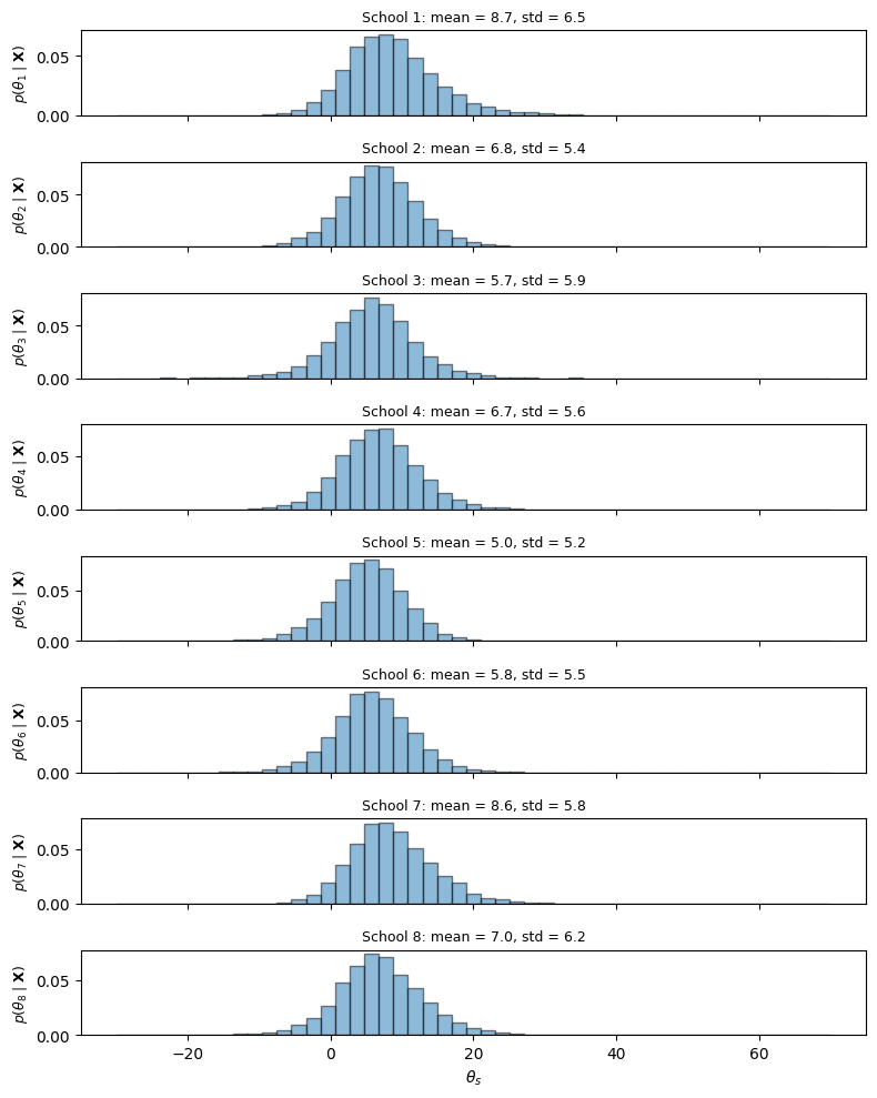

Comparison to Classical Analysis of Variance¶

A classical approach to estimating $\theta_s$ offers two extremes:

No pooling (unpooled): $\hat{\theta}_s = \bar{x}_s$ . Treat each school independently; ignore any similarity between schools.
Complete pooling: $\hat{\theta}_s = \bar{x}$ . Treat all schools as identical; pool all data.

An ANOVA F-test helps choose between them: if the between-group mean square is significantly larger than the within-group mean square, use unpooled estimates; otherwise use pooled.

The hierarchical Bayesian approach automatically interpolates between these extremes. The posterior mean $\E[\theta_s \mid \mbX]$ is a precision-weighted blend of the school mean $\bar{x}_s$ and the global mean $\hat{\mu}$ , with the blend determined by the posterior over $\tau^2$ . When $\tau^2$ is large (schools differ a lot), estimates are close to the unpooled $\bar{x}_s$ ; when $\tau^2$ is small (schools are similar), estimates shrink toward the pooled mean.

Two advantages of the Bayesian approach:

Uncertainty propagation. The posterior over $\theta_s$ reflects uncertainty about $\mu$ and $\tau^2$ , not just about $\theta_s$ given fixed global parameters. A plug-in estimate $\hat{\tau}^2$ underestimates posterior variance.
Coherence. The point estimate $\hat{\tau}^2 = (\mathrm{MS}_B - \mathrm{MS}_W)/N$ can be negative (set to zero in practice), which amounts to an overly strong claim that $\tau^2 = 0$ . The posterior remains well-behaved.

Conclusion¶

The hierarchical Gaussian model demonstrates exact Bayesian inference in a multi-level setting. The key steps were:

Express the joint posterior as a product $p(\mbtheta \mid \cdot)\, p(\mu \mid \tau^2, \cdot)\, p(\tau^2 \mid \cdot)$ using the product rule.
Compute $p(\mbtheta \mid \mu, \tau^2, \cdot)$ and $p(\mu \mid \tau^2, \cdot)$ analytically using linear Gaussian identities.
Evaluate and normalize $p(\tau^2 \mid \mbX)$ numerically on a 1D grid.
Draw samples from the joint posterior via ancestral sampling: sample $\tau \to \mu \to \mbtheta$ in the order implied by the factorization.

The posterior mean of each $\theta_s$ automatically partially pools the school estimate toward the global mean, with the degree of pooling governed by the posterior over $\tau^2$ .

Hierarchical Gaussian Models

Motivation¶

The Eight Schools Dataset¶

Bayesian Inference in the Hierarchical Gaussian Model¶

Step 1: Sufficient Statistics¶

Step 2: Per-School Posteriors (given μ\muμ and τ2\tau^2τ2)¶

Step 3: Posterior of the Global Mean (given τ2\tau^2τ2)¶

Step 4: Marginal Posterior of τ2\tau^2τ2¶

Step 5: Per-School Effects Marginalizing over μ\muμ¶

Posterior Sampling via Ancestral Sampling¶

Comparison to Classical Analysis of Variance¶

Conclusion¶

Step 2: Per-School Posteriors (given $\mu$ and $\tau^2$ )¶

Step 3: Posterior of the Global Mean (given $\tau^2$ )¶

Step 4: Marginal Posterior of $\tau^2$ ¶

Step 5: Per-School Effects Marginalizing over $\mu$ ¶