Topic Models

Mixture models assign each data point to a single component. But many real datasets are better described as mixtures of components within each data point. A document about climate policy draws from topics like “science”, “economics”, and “politics” simultaneously; a genome mixes ancestry from several populations.

Mixed membership models capture this by giving each data point its own distribution over components, rather than a single hard or soft assignment.

Latent Dirichlet Allocation (LDA) Blei et al., 2003 is the canonical mixed membership model for text. In this chapter we:

Define the general mixed membership model and the LDA special case
Derive Gibbs sampling and CAVI updates for LDA
Show why LDA tends to recover sharp topics
Work with the efficient word-count representation
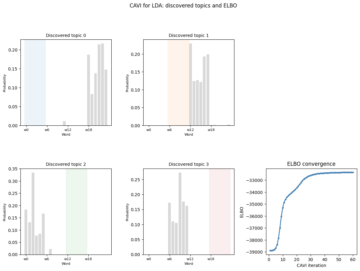
Implement CAVI for LDA and visualise recovered topics

import torch
import torch.distributions as dist
from torch.special import digamma
import matplotlib.pyplot as plt
import matplotlib.gridspec as gridspec
import numpy as np

palette = list(plt.cm.tab10.colors)

Mixed Membership Models¶

From Mixtures to Mixed Membership¶

In a mixture model every data point $\mbx_n$ is drawn from a single component $z_n \in \{1,\ldots,K\}$ . A mixed membership model relaxes this: each data point is itself a collection of observations $\mbx_n = (x_{n,1},\ldots,x_{n,D})$ , and different observations within the same data point can come from different components.

Applications:

Text: a document is a collection of words; different sentences may draw from different topics.
Social science: a survey respondent’s answers mix multiple viewpoints.
Genetics: a genome mixes ancestry from several populations Pritchard et al., 2000.

Notation¶

Symbol	Role
$N$	number of data points (documents)
$D$	observations per data point (words per document)
$K$	number of components (topics)
$V$	vocabulary size
$\mbtheta_k \in \Delta_{V-1}$	parameters of component $k$ (topic $k$ ’s distribution over words)
$\mbpi_n \in \Delta_{K-1}$	component proportions for data point $n$
$z_{n,d} \in \{1,\ldots,K\}$	assignment of observation $d$ in data point $n$
$x_{n,d} \in \{1,\ldots,V\}$	observed value (word index)

The key distinction from a mixture model: each data point has its own $\mbpi_n$ , rather than sharing a single global $\mbpi$ .

Topic Model Nomenclature¶

General	Topic model
data set	corpus
data point	document
observation	word
mixture component	topic
mixture proportions	topic proportions
assignment	topic assignment

Latent Dirichlet Allocation¶

LDA Blei et al., 2003 uses a fully conjugate Dirichlet–Categorical model for both topics and proportions.

Generative Process¶

\begin{aligned} \mbtheta_k &\overset{\text{iid}}{\sim} \operatorname{Dir}(\mbphi) && k = 1,\ldots,K \\ \mbpi_n &\overset{\text{iid}}{\sim} \operatorname{Dir}(\mbalpha) && n = 1,\ldots,N \\ z_{n,d} &\overset{\text{iid}}{\sim} \operatorname{Categorical}(\mbpi_n) && d = 1,\ldots,D \\ x_{n,d} &\sim \operatorname{Categorical}(\mbtheta_{z_{n,d}}) && d = 1,\ldots,D \end{aligned}

(1)

Joint Distribution¶

p\!\left(\{\mbtheta_k\},\{\mbpi_n, \mbz_n, \mbx_n\}\right) = \prod_{k=1}^K \operatorname{Dir}(\mbtheta_k \mid \mbphi) \prod_{n=1}^N \left[ \operatorname{Dir}(\mbpi_n \mid \mbalpha) \prod_{d=1}^D \pi_{n,z_{n,d}}\,\theta_{z_{n,d},\,x_{n,d}} \right].

(2)

Equivalently, in terms of count statistics

N_{n,k} = \sum_d \mathbb{I}[z_{n,d}=k], \qquad N_{k,v} = \sum_{n,d} \mathbb{I}[z_{n,d}=k]\,\mathbb{I}[x_{n,d}=v],

(3)

the joint factors into a product of Dirichlet terms:

p \propto \underbrace{\prod_{k,v} \theta_{k,v}^{\phi_v - 1}}_{\text{topic prior}} \prod_{n=1}^N \left( \underbrace{\prod_k \pi_{n,k}^{\alpha_k + N_{n,k} - 1}}_{\text{proportion prior + data}} \underbrace{\prod_{k,v} \theta_{k,v}^{N_{k,v}}}_{\text{topic likelihood}} \right).

(4)

Inference¶

Gibbs Sampling¶

For LDA all complete conditionals are Dirichlet or Categorical:

Topic assignments ( $z_{n,d}$ conditional on everything else):

p(z_{n,d} = k \mid x_{n,d} = v,\, \mbtheta_k,\, \mbpi_n) \propto \pi_{n,k}\, \theta_{k,v}.

(5)

Topic proportions ( $\mbpi_n$ conditional on assignments):

p(\mbpi_n \mid \mbalpha, \mbz_n) = \operatorname{Dir}\!\left(\alpha_1 + N_{n,1},\ldots,\alpha_K + N_{n,K}\right).

(6)

Topic parameters ( $\mbtheta_k$ conditional on all assignments and words):

p(\mbtheta_k \mid \mbphi, \{\mbz_n, \mbx_n\}) = \operatorname{Dir}\!\left( \phi_1 + \textstyle\sum_n N_{n,k,1},\;\ldots,\; \phi_V + \textstyle\sum_n N_{n,k,V} \right).

(7)

Why Does LDA Produce Sharp Topics?¶

The log-joint is dominated by the double sum over documents and words:

\sum_{n=1}^N \sum_{d=1}^D \bigl(\log \pi_{n,z_{n,d}} + \log \theta_{z_{n,d},x_{n,d}}\bigr).

(8)

Both $\mbpi_n$ and $\mbtheta_k$ live on a simplex, so maximising one term forces others down. The posterior balances two competing pressures:

Few topics per document: large $\pi_{n,k}$ for only a few $k$ .
Few words per topic: large $\theta_{k,v}$ for only a few $v$ .

The result is topics that concentrate on small, coherent word sets and documents that mix only a few of those topics.

CAVI for LDA¶

Variational Family¶

Following the CAVI recipe from the previous chapter, we use the mean-field family with factors matching the prior forms:

q = \underbrace{\prod_{k=1}^K \operatorname{Dir}(\mbtheta_k;\,\tilde{\mblambda}^{(\theta)}_k)}_{\text{topics}} \prod_{n=1}^N \left[ \underbrace{\operatorname{Dir}(\mbpi_n;\,\tilde{\mblambda}^{(\pi)}_n)}_{\text{proportions}} \prod_{d=1}^D \underbrace{\operatorname{Cat}(z_{n,d};\,\tilde{\mblambda}^{(z)}_{n,d})}_{\text{assignments}} \right].

(9)

Update for $q(z_{n,d})$ : Topic Assignments¶

\log q(z_{n,d}=k) = \mathbb{E}_{q(\mbpi_n)}[\log\pi_{n,k}] + \mathbb{E}_{q(\mbtheta_k)}[\log\theta_{k,x_{n,d}}] + c,

(10)

normalising to get:

\tilde{\lambda}^{(z)}_{n,d,k} \propto \exp\!\left\{ \mathbb{E}_q[\log\pi_{n,k}] + \mathbb{E}_q[\log\theta_{k,x_{n,d}}] \right\},

(11)

where the digamma expectations under a Dirichlet are:

\mathbb{E}_{\operatorname{Dir}(\mbalpha)}[\log\pi_k] = \psi(\alpha_k) - \psi\!\left(\textstyle\sum_j \alpha_j\right).

(12)

Update for $q(\mbpi_n)$ : Topic Proportions¶

\boxed{\tilde{\lambda}^{(\pi)}_{n,k} = \alpha_k + \sum_{d=1}^D \tilde{\lambda}^{(z)}_{n,d,k}.}

(13)

Update for $q(\mbtheta_k)$ : Topics¶

\boxed{\tilde{\lambda}^{(\theta)}_{k,v} = \phi_v + \sum_{n=1}^N \sum_{d=1}^D \tilde{\lambda}^{(z)}_{n,d,k}\,\mathbb{I}[x_{n,d}=v].}

(14)

Word-Count Representation¶

Since LDA models words as exchangeable, only the word counts $y_{n,v} = \sum_d \mathbb{I}[x_{n,d}=v]$ matter, not the word order. We replace the per-word variational parameters with per-type parameters:

\tilde{\lambda}^{(c)}_{n,v,k} \propto \exp\!\left\{\mathbb{E}_q[\log\pi_{n,k}] + \mathbb{E}_q[\log\theta_{k,v}]\right\},

(15)

and update the sufficient statistics as:

\mathbb{E}_q[N_{n,k}] = \sum_v y_{n,v}\,\tilde{\lambda}^{(c)}_{n,v,k}, \qquad \mathbb{E}_q[N_{k,v}] = \sum_n y_{n,v}\,\tilde{\lambda}^{(c)}_{n,v,k}.

(16)

This reduces the number of variational parameters from $N \times D \times K$ to $N \times V \times K$ (and only needs to be stored for non-zero word types, since $y_{n,v}=0$ contributes nothing).

ELBO for LDA¶

\mathcal{L} = \underbrace{\sum_{n,v} y_{n,v} \sum_k \tilde{\lambda}^{(c)}_{n,v,k} \bigl(\mathbb{E}_q[\log\pi_{n,k}] + \mathbb{E}_q[\log\theta_{k,v}]\bigr)}_{\text{expected log-likelihood + prior on }z} + \underbrace{\sum_{n,v} y_{n,v} H[\tilde{\mblambda}^{(c)}_{n,v,\cdot}]}_{\text{assignment entropy}} - \underbrace{\sum_k D_{\mathrm{KL}}\!\bigl(\operatorname{Dir}(\tilde{\mblambda}^{(\theta)}_k) \| \operatorname{Dir}(\mbphi)\bigr)}_{\text{KL for topics}} - \underbrace{\sum_n D_{\mathrm{KL}}\!\bigl(\operatorname{Dir}(\tilde{\mblambda}^{(\pi)}_n) \| \operatorname{Dir}(\mbalpha)\bigr).}_{\text{KL for proportions}}

(17)

# ── Synthetic corpus ─────────────────────────────────────────────────────────
torch.manual_seed(305)

V       = 24    # vocabulary size (6 words per topic)
K_true  = 4    # true number of topics
N       = 200  # documents
D       = 60   # words per document

# True topics: each concentrates on 6 consecutive words
φ_true = 0.05 * torch.ones(K_true, V)
for k in range(K_true):
    φ_true[k, k*6:(k+1)*6] = 10.0
θ_true = dist.Dirichlet(φ_true).sample()   # (K_true, V)

# True proportions: mild sparsity
α_true  = 0.5 * torch.ones(K_true)
π_true  = dist.Dirichlet(α_true).sample((N,))  # (N, K_true)

# Generate word-count matrix  y[n, v] = # occurrences of word v in doc n
y = torch.zeros(N, V, dtype=torch.float32)
for n in range(N):
    zs   = dist.Categorical(π_true[n]).sample((D,))       # (D,)
    words = torch.stack([dist.Categorical(θ_true[z]).sample() for z in zs])
    for v in range(V):
        y[n, v] = (words == v).sum().float()

print(f'Corpus: {N} docs, vocab size {V}, avg doc length {y.sum(1).mean():.1f}')
print(f'Vocabulary coverage: {(y > 0).float().mean():.2f} (fraction of doc-word pairs non-zero)')


# ── CAVI for LDA (word-count representation) ─────────────────────────────────
def cavi_lda(y, K, α, φ, num_iters=60, seed=0):
    """CAVI for LDA using the word-count representation.

    Parameters
    ----------
    y   : (N, V) word-count matrix
    K   : number of topics to fit
    α   : (K,) Dirichlet concentration for topic proportions
    φ   : (V,) Dirichlet concentration for topics
    """
    torch.manual_seed(seed)
    N, V = y.shape

    # ── Initialise ────────────────────────────────────────────────────────────
    # λ_z[n, v, k]  : soft topic assignments per word type (N, V, K)
    λ_z = torch.softmax(torch.randn(N, V, K), dim=2)

    # λ_pi[n, k]    : variational Dirichlet params for π_n (N, K)
    # λ_th[k, v]    : variational Dirichlet params for θ_k (K, V)
    def update_global(λ_z):
        # E_q[N_{n,k}] = Σ_v y[n,v] λ_z[n,v,k]
        E_N_nk  = (y.unsqueeze(2) * λ_z).sum(1)          # (N, K)
        # E_q[N_{k,v}] = Σ_n y[n,v] λ_z[n,v,k]
        E_N_kv  = (y.unsqueeze(2) * λ_z).sum(0).T        # (K, V)
        λ_pi = α.unsqueeze(0) + E_N_nk                   # (N, K)
        λ_th = φ.unsqueeze(0) + E_N_kv                   # (K, V)
        return λ_pi, λ_th

    def e_log_dir(λ):
        """E_Dir(λ)[log θ_k] = ψ(λ_k) - ψ(Σ λ_j), shape same as λ."""
        return digamma(λ) - digamma(λ.sum(-1, keepdim=True))

    def compute_elbo(y, λ_z, λ_pi, λ_th):
        E_lpi = e_log_dir(λ_pi)   # (N, K)
        E_lth = e_log_dir(λ_th)   # (K, V)

        # Expected log-likelihood + E[log p(z|π)]
        # Σ_{n,v} y[n,v] Σ_k λ_z[n,v,k] (E_lpi[n,k] + E_lth[k,v])
        lp_z  = E_lpi.unsqueeze(1) + E_lth.T.unsqueeze(0)   # (N, V, K)
        ell   = (y.unsqueeze(2) * λ_z * lp_z).sum()

        # Assignment entropy: Σ_{n,v} y[n,v] H[λ_z[n,v,:]]
        H_z   = -(λ_z * torch.log(λ_z.clamp(1e-40))).sum(2) # (N, V)
        h_ent = (y * H_z).sum()

        # KL for topics and proportions (use torch.distributions)
        kl_th = sum(
            dist.kl_divergence(dist.Dirichlet(λ_th[k]), dist.Dirichlet(φ)).item()
            for k in range(K))
        kl_pi = sum(
            dist.kl_divergence(dist.Dirichlet(λ_pi[n]), dist.Dirichlet(α)).item()
            for n in range(N))

        return (ell + h_ent - kl_th - kl_pi).item()

    # ── CAVI loop ─────────────────────────────────────────────────────────────
    elbos = []
    for _ in range(num_iters):
        # Update global params
        λ_pi, λ_th = update_global(λ_z)

        # Update topic assignments (local step)
        E_lpi = e_log_dir(λ_pi)   # (N, K)
        E_lth = e_log_dir(λ_th)   # (K, V)
        log_λ_z = E_lpi.unsqueeze(1) + E_lth.T.unsqueeze(0)  # (N, V, K)
        λ_z = torch.softmax(log_λ_z, dim=2)

        elbos.append(compute_elbo(y, λ_z, λ_pi, λ_th))

    λ_pi, λ_th = update_global(λ_z)
    return λ_pi, λ_th, λ_z, elbos


K   = 4
α   = 0.5 * torch.ones(K)
φ   = 0.1 * torch.ones(V)

λ_pi, λ_th, λ_z, elbos = cavi_lda(y, K=K, α=α, φ=φ, num_iters=60)

# Posterior mean topics
θ_hat = λ_th / λ_th.sum(1, keepdim=True)   # (K, V)
print('\nTop 3 words per discovered topic:')
for k in range(K):
    top = θ_hat[k].topk(3).indices.tolist()
    print(f'  Topic {k}: words {top}  (true topic words: {list(range(k*6, k*6+6))}'
          f' if k matches)')

Corpus: 200 docs, vocab size 24, avg doc length 60.0
Vocabulary coverage: 0.64 (fraction of doc-word pairs non-zero)


Top 3 words per discovered topic:
  Topic 0: words [22, 21, 18]  (true topic words: [0, 1, 2, 3, 4, 5] if k matches)
  Topic 1: words [12, 17, 16]  (true topic words: [6, 7, 8, 9, 10, 11] if k matches)
  Topic 2: words [2, 0, 5]  (true topic words: [12, 13, 14, 15, 16, 17] if k matches)
  Topic 3: words [9, 10, 6]  (true topic words: [18, 19, 20, 21, 22, 23] if k matches)

fig = plt.figure(figsize=(14, 9))
gs  = gridspec.GridSpec(2, 3, figure=fig, hspace=0.45, wspace=0.35)

word_labels = [f'w{v}' for v in range(V)]
topic_colors = [palette[k] for k in range(K)]

# ── Top row: discovered topics ───────────────────────────────────────────────
for k in range(K):
    ax = fig.add_subplot(gs[0, k] if K <= 3 else gs[k // 2, k % 2 + (1 if k >= 2 else 0)])
    # Reuse a 2×2 layout
    ax = fig.add_subplot(gs[0, k] if k < 3 else gs[1, 0])

# Redo with a proper 2×2 for topics
for spine in fig.axes:
    spine.remove()
fig.clf()
gs = gridspec.GridSpec(2, 3, figure=fig, hspace=0.5, wspace=0.35)

# Topics
for k in range(K):
    r, c = divmod(k, 2)
    ax = fig.add_subplot(gs[r, c])
    vals = θ_hat[k].numpy()
    bars = ax.bar(range(V), vals, color=[
        palette[k] if (k2 == k) else 'lightgray'
        for k2 in [v // 6 for v in range(V)]
    ], alpha=0.85)
    ax.set_xticks(range(0, V, 6))
    ax.set_xticklabels([f'w{v}' for v in range(0, V, 6)], fontsize=8)
    ax.set_title(f'Discovered topic {k}', fontsize=10)
    ax.set_ylabel('Probability', fontsize=8)
    ax.set_xlabel('Word', fontsize=8)
    # Mark words belonging to this topic
    ax.axvspan(k*6 - 0.5, k*6 + 5.5, alpha=0.08, color=palette[k])

# ELBO convergence
ax_elbo = fig.add_subplot(gs[1, 2])
ax_elbo.plot(range(1, len(elbos)+1), elbos, 'o-', color='steelblue', ms=3, lw=2)
ax_elbo.set_xlabel('CAVI iteration')
ax_elbo.set_ylabel('ELBO')
ax_elbo.set_title('ELBO convergence')

plt.suptitle('CAVI for LDA: discovered topics and ELBO', fontsize=12, y=1.01)
plt.tight_layout()

/tmp/ipykernel_2526/541953727.py:44: UserWarning: This figure includes Axes that are not compatible with tight_layout, so results might be incorrect.
  plt.tight_layout()

# Posterior mean topic proportions for a sample of documents
π_hat = λ_pi / λ_pi.sum(1, keepdim=True)   # (N, K)

fig, axes = plt.subplots(1, 2, figsize=(12, 4))

# Left: stacked bar of topic proportions for 20 documents
ax = axes[0]
n_show = 30
bottom = torch.zeros(n_show)
for k in range(K):
    vals = π_hat[:n_show, k].numpy()
    ax.bar(range(n_show), vals, bottom=bottom.numpy(),
           color=palette[k], label=f'Topic {k}', alpha=0.85)
    bottom = bottom + torch.tensor(vals)
ax.set_xlabel('Document index')
ax.set_ylabel('Topic proportion')
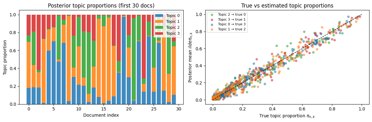
ax.set_title('Posterior topic proportions (first 30 docs)')
ax.legend(fontsize=9, loc='upper right')

# Right: scatter of true vs estimated proportions for topic 0 vs topic 1
ax = axes[1]
# Try to match discovered topics to true topics by top word overlap
def match_topic(θ_hat, θ_true):
    """Greedy matching of discovered topics to true topics by cosine sim."""
    K = θ_hat.shape[0]
    sim = θ_hat @ θ_true.T   # (K, K_true)
    matched = {}
    used = set()
    for _ in range(K):
        i, j = (sim * torch.tensor([[1.0 if j not in used else 0.0
                                      for j in range(K)] for i in range(K)]
                                   )).argmax().item(), None
        i, j = divmod(i, K)
        matched[i] = j
        used.add(j)
    return matched

match = match_topic(θ_hat, θ_true)
# Plot true vs posterior mean for each topic
for k, k_true in match.items():
    ax.scatter(π_true[:, k_true].numpy(), π_hat[:, k].numpy(),
               alpha=0.5, s=20, color=palette[k],
               label=f'Topic {k} → true {k_true}')
ax.plot([0, 1], [0, 1], 'k--', lw=1)
ax.set_xlabel('True topic proportion $\pi_{n,k}$')
ax.set_ylabel('Posterior mean $\tilde{\pi}_{n,k}$')
ax.set_title('True vs estimated topic proportions')
ax.legend(fontsize=8)

plt.tight_layout()

<>:45: SyntaxWarning: invalid escape sequence '\p'
<>:46: SyntaxWarning: invalid escape sequence '\p'
<>:45: SyntaxWarning: invalid escape sequence '\p'
<>:46: SyntaxWarning: invalid escape sequence '\p'
/tmp/ipykernel_2526/848507839.py:45: SyntaxWarning: invalid escape sequence '\p'
  ax.set_xlabel('True topic proportion $\pi_{n,k}$')
/tmp/ipykernel_2526/848507839.py:46: SyntaxWarning: invalid escape sequence '\p'
  ax.set_ylabel('Posterior mean $\tilde{\pi}_{n,k}$')

Scaling and Evaluation¶

Stochastic Variational Inference¶

For large corpora (millions of documents), CAVI over the full corpus is expensive. Stochastic Variational Inference (SVI) Hoffman et al., 2013 scales it to mini-batches:

Sample a mini-batch $\mathcal{B}$ of documents.
Run the local CAVI updates (assignments $\tilde{\lambda}^{(c)}_{n,v,k}$ and proportions $\tilde{\lambda}^{(\pi)}_n$ ) for $n \in \mathcal{B}$ .
Scale up the expected word counts and take a natural gradient step on the global topic parameters $\tilde{\lambda}^{(\theta)}_k$ .

Because the ELBO is a sum over documents, the mini-batch provides an unbiased (if noisy) natural gradient, and the update has the same closed form as full CAVI but on the mini-batch.

Evaluating Topic Models: Held-Out Likelihood¶

Comparing ELBO values for different $K$ is problematic — the ELBO is a lower bound, not the true marginal likelihood, so it cannot be reliably used for model selection.

Wallach et al., 2009 recommend evaluating on held-out documents: split each new document $n'$ into an in portion $\mbx_{n'}^{\mathsf{in}}$ (used to infer $\mbpi_{n'}$ with fixed topics) and an out portion $\mbx_{n'}^{\mathsf{out}}$ (used to evaluate predictive likelihood):

p(\mbx_{n'}^{\mathsf{out}} \mid \mbx_{n'}^{\mathsf{in}}, \{\mbx_n\}) = \int p(\mbx_{n'}^{\mathsf{out}} \mid \mbpi_{n'}, \{\mbtheta_k\})\, p(\mbpi_{n'} \mid \mbx_{n'}^{\mathsf{in}}, \{\mbtheta_k\})\, p(\{\mbtheta_k\} \mid \{\mbx_n\})\;d\mbpi_{n'}.

(18)

This measures whether the model can predict unseen words given the observed context — a proper generalisation test.

Other Mixed Membership Models¶

The mixed membership idea extends far beyond text:

Population genetics Pritchard et al., 2000: genomes mix ancestry from $K$ populations.
Survey data Erosheva et al., 2007: respondents mix $K$ latent profiles.
Community detection Airoldi et al., 2008: network nodes have mixed membership across $K$ communities.
Poisson matrix factorisation Gopalan et al., 2013: a Poisson likelihood variant of LDA with applications to recommendation systems.

Conclusion¶

Mixed membership models extend mixture models by allowing each data point to draw from multiple components through its own per-document topic proportions $\mbpi_n$ .

	Mixture model	Mixed membership (LDA)
Latent variable per item	$z_n \in \{1,\ldots,K\}$	$\mbpi_n \in \Delta_{K-1}$
Latent variable per observation	—	$z_{n,d} \in \{1,\ldots,K\}$
Component parameters	shared $\{\mbtheta_k\}$	shared $\{\mbtheta_k\}$
CAVI updates	3 factors	3 factors + local $z_{n,d}$ per word

Key takeaways:

CAVI updates for LDA have the same Dirichlet conjugate form as before, but the sufficient statistics $N_{n,k}$ and $N_{k,v}$ are now weighted sums of soft topic assignments rather than hard counts.
The digamma correction $\psi(\tilde{\lambda}_k) - \psi(\sum_j \tilde{\lambda}_j)$ replaces $\log \pi_{n,k}$ and $\log \theta_{k,v}$ everywhere, propagating uncertainty about the Dirichlet parameters.
The word-count representation collapses $N \times D \times K$ assignment variables to $N \times V \times K$ , exploiting exchangeability.
LDA produces sharp topics because maximising both $\log \pi_{n,k}$ and $\log \theta_{k,v}$ simultaneously forces each to concentrate.
SVI scales CAVI to large corpora via mini-batch natural gradient steps.

References¶

Blei, D. M., Ng, A. Y., & Jordan, M. I. (2003). Latent Dirichlet allocation. Journal of Machine Learning Research, 3, 993–1022.
Pritchard, J. K., Stephens, M., & Donnelly, P. (2000). Inference of population structure using multilocus genotype data. Genetics, 155(2), 945–959.
Hoffman, M. D., Blei, D. M., Wang, C., & Paisley, J. (2013). Stochastic variational inference. Journal of Machine Learning Research, 14(5).
Wallach, H. M., Murray, I., Salakhutdinov, R., & Mimno, D. (2009). Evaluation methods for topic models. Proceedings of the 26th Annual International Conference on Machine Learning, 1105–1112.
Erosheva, E. A., Fienberg, S. E., & Joutard, C. (2007). DESCRIBING DISABILITY THROUGH INDIVIDUAL-LEVEL MIXTURE MODELS For MULTIVARIATE BINARY DATA. Ann. Appl. Stat., 1(2), 346–384.
Airoldi, E. M., Blei, D. M., Fienberg, S. E., & Xing, E. P. (2008). Mixed Membership Stochastic Blockmodels. J. Mach. Learn. Res., 9, 1981–2014.
Gopalan, P., Hofman, J. M., & Blei, D. M. (2013). Scalable Recommendation with Poisson Factorization.
Blei, D. M. (2012). Probabilistic topic models. Communications of the ACM, 55(4), 77–84.

Mixed Membership Models¶

From Mixtures to Mixed Membership¶

Notation¶

Topic Model Nomenclature¶

Latent Dirichlet Allocation¶

Generative Process¶

Joint Distribution¶

Inference¶

Gibbs Sampling¶

Why Does LDA Produce Sharp Topics?¶

CAVI for LDA¶

Variational Family¶

Update for q(zn,d)q(z_{n,d})q(zn,d​): Topic Assignments¶

Update for q(πn)q(\mbpi_n)q(πn​): Topic Proportions¶

Update for q(θk)q(\mbtheta_k)q(θk​): Topics¶

Word-Count Representation¶

ELBO for LDA¶

Scaling and Evaluation¶

Stochastic Variational Inference¶

Evaluating Topic Models: Held-Out Likelihood¶

Other Mixed Membership Models¶

Conclusion¶

Update for $q(z_{n,d})$ : Topic Assignments¶

Update for $q(\mbpi_n)$ : Topic Proportions¶

Update for $q(\mbtheta_k)$ : Topics¶