Coordinate Ascent Variational Inference

In the previous chapter we used EM to find point estimates of the parameters $\{\mbmu_k, \mbpi\}$ while computing exact posteriors over the discrete assignments $\{z_n\}$ . But EM does not give us uncertainty over the parameters themselves.

Variational inference (VI) takes a different approach: instead of sampling from the posterior (MCMC) or computing it exactly (conjugate inference), we approximate it with a tractable parametric distribution $q(\mbtheta; \mblambda)$ and optimise the variational parameters $\mblambda$ to make the approximation as close as possible to the true posterior.

Coordinate Ascent Variational Inference (CAVI) is the simplest VI algorithm:

Family: the mean-field factorisation $q(\mbtheta) = \prod_j q(\theta_j)$
Divergence: the KL divergence $D_{\mathrm{KL}}(q \| p)$
Optimisation: coordinate ascent over each factor in turn

Topics covered:

Motivation: VI vs MCMC
The mean-field family and the ELBO as a KL objective
General CAVI update formula
Full derivation for the Gaussian mixture model (GMM)
Computing the ELBO for the GMM
Code: CAVI for the GMM with ELBO tracking and posterior uncertainty

import torch
import torch.distributions as dist
from torch.special import digamma
import matplotlib.pyplot as plt
import matplotlib.patches as mpatches
from matplotlib.patches import Ellipse

palette = list(plt.cm.tab10.colors)

Motivation: Why Variational Inference?¶

We have seen several posterior inference algorithms:

Algorithm	Pros	Cons
Conjugate inference	Exact; closed form	Only for conjugate models
Gibbs sampling	Flexible; asymptotically exact	Slow mixing; high variance
HMC	Handles complex continuous posteriors	Requires gradient; expensive
EM	Fast; closed-form updates	Only point estimates of parameters

MCMC methods are asymptotically unbiased — given infinite samples they converge to the true posterior. But in practice, with finite computation, the variance of MCMC estimators decays only as $O(S^{-1/2})$ .

Key question: Can we trade a small asymptotic bias for much lower variance and faster computation?

Variational inference says yes: approximate the posterior with a tractable family, optimise to minimise the approximation error, then use the fitted approximation as a surrogate for the posterior.

VI converts inference into optimisation, which tends to be faster and easier to scale than sampling.

The Variational Inference Framework¶

Notation¶

Let $\mbtheta$ denote all latent variables and parameters we wish to infer. For the GMM:

\mbtheta = \bigl(\mbpi,\; \{\mbmu_k\}_{k=1}^K,\; \{z_n\}_{n=1}^N\bigr).

(1)

Note that unlike EM, VI gives a full posterior over both the parameters $(\mbpi, \{\mbmu_k\})$ and the latent variables $\{z_n\}$ .

Let $q(\mbtheta; \mblambda)$ denote the variational approximation with variational parameters $\mblambda$ , and let $p(\mbtheta \mid \mbx)$ be the true (intractable) posterior.

Objective: KL Divergence¶

We measure closeness with the reverse KL divergence:

D_{\mathrm{KL}}\bigl(q(\mbtheta; \mblambda) \,\|\, p(\mbtheta \mid \mbx)\bigr) = \mathbb{E}_{q}\!\left[\log \frac{q(\mbtheta; \mblambda)}{p(\mbtheta \mid \mbx)}\right].

(2)

The posterior $p(\mbtheta \mid \mbx)$ is intractable (requires the evidence $p(\mbx)$ ). But we can rewrite the KL in terms of the log joint:

D_{\mathrm{KL}}(q \| p) = \underbrace{\mathbb{E}_q[\log q(\mbtheta; \mblambda)] - \mathbb{E}_q[\log p(\mbtheta, \mbx)]}_{-\mathcal{L}(\mblambda)} + \log p(\mbx).

(3)

Since $\log p(\mbx)$ does not depend on $\mblambda$ , minimising the KL is equivalent to maximising the ELBO:

\mathcal{L}(\mblambda) = \mathbb{E}_q[\log p(\mbtheta, \mbx)] - \mathbb{E}_q[\log q(\mbtheta; \mblambda)] \leq \log p(\mbx).

(4)

The ELBO lower-bounds the log evidence — hence its name.

The Mean-Field Family¶

The mean-field family factorises the variational posterior over each variable:

q(\mbtheta; \mblambda) = \prod_{j=1}^J q(\theta_j; \lambda_j).

(5)

This ignores posterior correlations between variables but makes the optimisation tractable.

The CAVI Update¶

With the mean-field factorisation, we can optimise each factor $q(\theta_j; \lambda_j)$ while holding all others fixed.

As a function of $\lambda_j$ alone, the ELBO is:

\mathcal{L}(\mblambda) = \mathbb{E}_{q(\theta_j)}\!\left[ \underbrace{\mathbb{E}_{q(\mbtheta_{\neg j})}[\log p(\theta_j \mid \mbtheta_{\neg j}, \mbx)]}_{\triangleq\, \log \tilde{p}(\theta_j)} \right] - \mathbb{E}_{q(\theta_j)}[\log q(\theta_j; \lambda_j)] + c = -D_{\mathrm{KL}}\bigl(q(\theta_j) \,\|\, \tilde{p}(\theta_j)\bigr) + c,

(6)

where the unnormalised target is:

\boxed{\log \tilde{p}(\theta_j) \propto \mathbb{E}_{q(\mbtheta_{\neg j})}\!\left[\log p(\theta_j \mid \mbtheta_{\neg j}, \mbx)\right].}

(7)

The KL is minimised when $q(\theta_j; \lambda_j^\star) = \tilde{p}(\theta_j)$ . So the optimal CAVI update sets $q(\theta_j)$ proportional to the exponentiated expected log conditional of $\theta_j$ given everything else.

CAVI for Gaussian Mixture Models¶

Variational Family¶

Assume the mean-field approximation with factors of the same exponential family form as the priors:

q(\mbtheta; \mblambda) = \underbrace{q(\mbpi;\, \tilde{\mbalpha})}_{\mathrm{Dirichlet}} \prod_{k=1}^K \underbrace{q(\mbmu_k;\, \tilde{\nu}_k, \tilde{\mbphi}_k)}_{\mathrm{Gaussian}} \prod_{n=1}^N \underbrace{q(z_n;\, \tilde{\mbomega}_n)}_{\mathrm{Categorical}},

(8)

where the variational parameters are $\mblambda = (\tilde{\mbalpha},\; \{\tilde{\nu}_k, \tilde{\mbphi}_k\},\; \{\tilde{\mbomega}_n\})$ .

(For conjugate exponential-family models, the optimal variational factors always have the same form as the corresponding priors — so this choice is not an approximation, just a parameterisation.)

Update for $q(z_n)$ : Responsibilities¶

Applying the CAVI formula to $z_n$ :

\log q(z_n = k;\, \tilde{\mbomega}_n) = \mathbb{E}_{q(\mbpi)}[\log \pi_k] + \mathbb{E}_{q(\mbmu_k)}[\log \mathcal{N}(\mbx_n \mid \mbmu_k, \mbI)] + c.

(9)

Normalising over $k$ gives:

\tilde{\omega}_{n,k} = \frac{\exp\!\left\{\mathbb{E}_q[\log \pi_k] + \mathbb{E}_q[\log \mathcal{N}(\mbx_n \mid \mbmu_k, \mbI)]\right\}}{\sum_{j=1}^K \exp\!\left\{\mathbb{E}_q[\log \pi_j] + \mathbb{E}_q[\log \mathcal{N}(\mbx_n \mid \mbmu_j, \mbI)]\right\}}.

(10)

Computing the two expectations:

1. Expectation of log proportions under Dirichlet:

\mathbb{E}_{\mathrm{Dir}(\mbpi;\, \tilde{\mbalpha})}[\log \pi_k] = \psi(\tilde{\alpha}_k) - \psi\!\left(\sum_{j=1}^K \tilde{\alpha}_j\right),

(11)

where $\psi$ is the digamma function $\psi(x) = \frac{d}{dx}\log\Gamma(x)$ .

2. Gaussian cross-entropy under the variational mean:

Under $q(\mbmu_k) = \mathcal{N}(\tilde{\mbmu}_k, \tilde{\nu}_k^{-1}\mbI)$ (where $\tilde{\mbmu}_k = \tilde{\mbphi}_k / \tilde{\nu}_k$ ):

\mathbb{E}_{q(\mbmu_k)}[\log \mathcal{N}(\mbx_n \mid \mbmu_k, \mbI)] = \log \mathcal{N}(\mbx_n \mid \tilde{\mbmu}_k, \mbI) - \frac{D}{2\tilde{\nu}_k}.

(12)

The correction $-D/(2\tilde{\nu}_k)$ accounts for uncertainty in $\mbmu_k$ : when $\tilde{\nu}_k$ is small (high uncertainty), the effective likelihood is weaker.

Update for $q(\mbpi)$ : Dirichlet¶

\log q(\mbpi;\, \tilde{\mbalpha}) = \log p(\mbpi \mid \mbalpha) + \sum_{n=1}^N \sum_{k=1}^K \tilde{\omega}_{n,k} \log \pi_k + c \;\Rightarrow\; \boxed{\tilde{\alpha}_k = \alpha_k + \sum_{n=1}^N \tilde{\omega}_{n,k}.}

(13)

Update for $q(\mbmu_k)$ : Gaussian¶

\log q(\mbmu_k;\, \tilde{\nu}_k, \tilde{\mbphi}_k) = \log p(\mbmu_k \mid \mbphi, \nu) + \sum_{n=1}^N \tilde{\omega}_{n,k} \log \mathcal{N}(\mbx_n \mid \mbmu_k, \mbI) + c,

(14)

which gives a Gaussian with updated natural parameters:

\boxed{\tilde{\nu}_k = \nu + N_k, \qquad \tilde{\mbphi}_k = \mbphi + \sum_{n=1}^N \tilde{\omega}_{n,k}\,\mbx_n,}

(15)

where $N_k = \sum_n \tilde{\omega}_{n,k}$ . The posterior mean is $\tilde{\mbmu}_k = \tilde{\mbphi}_k / \tilde{\nu}_k$ .

The ELBO for the Gaussian Mixture Model¶

Expanding the ELBO using the mean-field factorisation:

\mathcal{L}(\mblambda) = \underbrace{\sum_{n=1}^N \sum_{k=1}^K \tilde{\omega}_{n,k}\, \mathbb{E}_{q(\mbmu_k)}\!\left[\log \mathcal{N}(\mbx_n \mid \mbmu_k, \mbI)\right]}_{\text{expected log-likelihood}} + \underbrace{\sum_{n=1}^N \sum_{k=1}^K \tilde{\omega}_{n,k}\, \mathbb{E}_{q(\mbpi)}[\log \pi_k]}_{\text{expected log-prior on }z} + \underbrace{\sum_{n=1}^N H[q(z_n)]}_{\text{entropy of assignments}} - \underbrace{\sum_{k=1}^K D_{\mathrm{KL}}\bigl(q(\mbmu_k) \,\|\, p(\mbmu_k)\bigr)}_{\text{KL for means}} - \underbrace{D_{\mathrm{KL}}\bigl(q(\mbpi) \,\|\, p(\mbpi)\bigr).}_{\text{KL for proportions}}

(16)

Each term has a closed form:

Expected log-likelihood: sum of $\tilde{\omega}_{n,k}[\log \mathcal{N}(\mbx_n \mid \tilde{\mbmu}_k, \mbI) - D/(2\tilde{\nu}_k)]$
Entropy of $q(z_n)$ : $H = -\sum_k \tilde{\omega}_{n,k} \log \tilde{\omega}_{n,k}$
KL for Gaussians: $D_{\mathrm{KL}}(\mathcal{N}(\tilde{\mbmu}_k, \tilde{\nu}_k^{-1}\mbI) \| \mathcal{N}(\nu^{-1}\mbphi, \nu^{-1}\mbI))$ in closed form
KL for Dirichlet: $D_{\mathrm{KL}}(\mathrm{Dir}(\tilde{\mbalpha}) \| \mathrm{Dir}(\mbalpha))$ in closed form

CAVI is guaranteed to increase the ELBO (or leave it unchanged) at each coordinate update, and the sequence of ELBO values converges.

# ── Data ─────────────────────────────────────────────────────────────────────
torch.manual_seed(305)
N, K, D = 300, 3, 2

π_true = torch.tensor([0.3, 0.4, 0.3])
μ_true = torch.tensor([[-3., -1.], [1., 3.], [3., -2.]])
z_true = dist.Categorical(π_true).sample((N,))
x = μ_true[z_true] + torch.randn(N, D)


def cavi_gmm(x, K, α, ν, φ, num_iters=50, seed=0):
    """Coordinate Ascent Variational Inference for a unit-variance GMM.

    Priors:
        π | α   ~ Dir(α)                    α: (K,)
        μ_k | ν, φ ~ N(φ/ν, I/ν)           ν: scalar, φ: (D,)

    Variational family:
        q(π)      = Dir(α̃)
        q(μ_k)    = N(φ̃_k/ν̃_k, I/ν̃_k)
        q(z_n)    = Categorical(ω̃_n)

    Returns variational parameters and ELBO history.
    """
    torch.manual_seed(seed)
    N, D = x.shape

    # ── Initialise ────────────────────────────────────────────────────────────
    # Random soft assignments
    ω̃ = torch.softmax(torch.randn(N, K), dim=1)   # (N, K)

    # Helper: update global parameters from current ω̃
    def update_global(ω̃):
        N_k   = ω̃.sum(0)                           # (K,)
        α̃     = α + N_k
        ν̃     = ν + N_k                             # (K,)
        φ̃     = φ.unsqueeze(0) + ω̃.T @ x           # (K, D)
        return α̃, ν̃, φ̃

    def e_log_pi(α̃):
        """E_Dir(α̃)[log π_k] = ψ(α̃_k) - ψ(Σ α̃_j)"""
        return digamma(α̃) - digamma(α̃.sum())       # (K,)

    def e_log_lik(x, ν̃, φ̃):
        """E_{q(μ_k)}[log N(x_n | μ_k, I)] for all n, k.

        = log N(x_n | μ̃_k, I) - D / (2 ν̃_k)
        """
        μ̃ = φ̃ / ν̃.unsqueeze(1)                    # (K, D)
        # log N(x_n | μ̃_k, I): shape (N, K)
        diff  = x.unsqueeze(1) - μ̃.unsqueeze(0)    # (N, K, D)
        log_n = -0.5 * (diff ** 2).sum(-1) - (D / 2) * torch.log(torch.tensor(2 * torch.pi))
        correction = D / (2 * ν̃)                   # (K,)
        return log_n - correction.unsqueeze(0)      # (N, K)

    def compute_elbo(x, ω̃, α̃, ν̃, φ̃):
        """Compute the ELBO."""
        μ̃  = φ̃ / ν̃.unsqueeze(1)                    # (K, D)
        μ0 = φ / ν

        # Expected log-likelihood term
        ell = (ω̃ * e_log_lik(x, ν̃, φ̃)).sum()

        # Expected log p(z | π) = Σ_n Σ_k ω̃_{nk} E[log π_k]
        elp_z = (ω̃ * e_log_pi(α̃).unsqueeze(0)).sum()

        # Entropy of q(z_n) = Σ_n H[Categorical(ω̃_n)]
        H_z = -(ω̃ * torch.log(ω̃.clamp(min=1e-40))).sum()

        # KL[ q(μ_k) || p(μ_k) ] summed over k — use torch.distributions
        kl_mu = sum(
            dist.kl_divergence(
                dist.MultivariateNormal(μ̃[k], (1 / ν̃[k]) * torch.eye(D)),
                dist.MultivariateNormal(μ0,   (1 / ν)     * torch.eye(D)),
            ).item()
            for k in range(K)
        )

        # KL[ q(π) || p(π) ]
        kl_pi = dist.kl_divergence(dist.Dirichlet(α̃), dist.Dirichlet(α)).item()

        return (ell + elp_z + H_z - kl_mu - kl_pi).item()

    # ── CAVI loop ─────────────────────────────────────────────────────────────
    elbos = []
    for _ in range(num_iters):
        # Update global variational parameters
        α̃, ν̃, φ̃ = update_global(ω̃)

        # Update q(z_n): responsibilities
        log_ω = e_log_pi(α̃).unsqueeze(0) + e_log_lik(x, ν̃, φ̃)   # (N, K)
        ω̃ = torch.softmax(log_ω, dim=1)

        elbos.append(compute_elbo(x, ω̃, α̃, ν̃, φ̃))

    # Final global update
    α̃, ν̃, φ̃ = update_global(ω̃)
    return α̃, ν̃, φ̃, ω̃, elbos


# Prior hyperparameters
α = torch.ones(K)                       # symmetric Dirichlet
ν = torch.tensor(1.0)                   # weak prior precision on means
φ = torch.zeros(D)                      # prior mean = 0

α̃, ν̃, φ̃, ω̃, elbos = cavi_gmm(x, K=K, α=α, ν=ν, φ=φ, num_iters=50)

μ̃ = φ̃ / ν̃.unsqueeze(1)
π̃ = (α̃ - 1) / (α̃ - 1).sum()    # approximate mode of Dirichlet
print('Posterior mean of cluster means:')
for k in range(K):
    print(f'  k={k}: μ̃={μ̃[k].numpy().round(2)},  '
          f'std={1/ν̃[k].sqrt().item():.3f},  π̃≈{π̃[k].item():.2f}')

Posterior mean of cluster means:
  k=0: μ̃=[-2.85 -0.92],  std=0.108,  π̃≈0.28
  k=1: μ̃=[ 2.92 -1.98],  std=0.103,  π̃≈0.31
  k=2: μ̃=[1.06 3.1 ],  std=0.090,  π̃≈0.41

def plot_cov_ellipse(ax, mean, cov, n_std=2, **kwargs):
    """Plot a covariance ellipse at n_std standard deviations."""
    vals, vecs = torch.linalg.eigh(cov)
    angle = torch.atan2(vecs[1, 0], vecs[0, 0]).item() * 180 / 3.14159
    w, h = 2 * n_std * vals.sqrt().numpy()
    ell = Ellipse(xy=mean.numpy(), width=w, height=h, angle=angle, **kwargs)
    ax.add_patch(ell)


fig, axes = plt.subplots(1, 3, figsize=(14, 4))

# ── Panel 1: CAVI soft assignments ───────────────────────────────────────────
ax = axes[0]
colors = (ω̃.numpy()[:, :, None] * torch.tensor([palette[k] for k in range(K)]).numpy()).sum(1)
ax.scatter(x[:, 0].numpy(), x[:, 1].numpy(), c=colors, s=18, alpha=0.7)
for k in range(K):
    post_cov = (1 / ν̃[k]) * torch.eye(D)
    plot_cov_ellipse(ax, μ̃[k], post_cov, n_std=2,
                     edgecolor=palette[k], facecolor='none', lw=2, ls='--', zorder=5)
    ax.scatter(*μ̃[k].numpy(), marker='*', s=300, color=palette[k],
               edgecolors='black', lw=0.8, zorder=6, label=f'k={k+1}')
ax.set_xlabel(r'$x_1$'); ax.set_ylabel(r'$x_2$')
ax.set_title('CAVI: soft assignments\n(dashed = 2σ posterior on μ)')
ax.legend(fontsize=9)

# ── Panel 2: True means vs CAVI posterior means ───────────────────────────────
ax = axes[1]
ax.scatter(x[:, 0].numpy(), x[:, 1].numpy(), color='lightgray', s=10, alpha=0.4)
for k in range(K):
    ax.scatter(*μ_true[k].numpy(), marker='D', s=180,
               color=palette[k], edgecolors='black', lw=0.8, zorder=6,
               label='True' if k == 0 else '_')
    post_cov = (1 / ν̃[k]) * torch.eye(D)
    plot_cov_ellipse(ax, μ̃[k], post_cov, n_std=2,
                     edgecolor=palette[k], facecolor=(*palette[k], 0.15), lw=2, zorder=5)
    ax.scatter(*μ̃[k].numpy(), marker='*', s=280,
               color=palette[k], edgecolors='black', lw=0.8, zorder=7,
               label='CAVI' if k == 0 else '_')
ax.set_xlabel(r'$x_1$'); ax.set_ylabel(r'$x_2$')
ax.set_title('True means (◆) vs CAVI posterior means (★)\nshaded = 2σ posterior uncertainty')
ax.legend(fontsize=9)

# ── Panel 3: ELBO convergence ────────────────────────────────────────────────
axes[2].plot(range(1, len(elbos)+1), elbos, 'o-', color='steelblue', ms=4, lw=2)
axes[2].set_xlabel('CAVI iteration')
axes[2].set_ylabel(r'ELBO $\mathcal{L}(\tilde{\boldsymbol{\lambda}})$')
axes[2].set_title('ELBO convergence')

plt.tight_layout()

Demo: CAVI versus MCMC for a Gaussian Model¶

To build intuition about the bias–variance tradeoff between variational inference and MCMC, we apply CAVI to a simple two-parameter model where the exact posterior is also available in closed form.

Model. A Gaussian with unknown mean and variance under a normal-inverse- $\chi^2$ (NIX) conjugate prior:

\sigma^2 \sim \chi^{-2}(\nu_0,\, \sigma_0^2), \qquad \mu \mid \sigma^2 \sim \mathcal{N}\!(\mu_0,\, \kappa_0^{-1}\sigma^2), \qquad x_n \mid \mu, \sigma^2 \overset{\text{iid}}{\sim} \mathcal{N}\!(\mu, \sigma^2).

(17)

The true posterior is NIX with closed-form hyperparameters, but it is not mean-field: $\mu$ and $\sigma^2$ are coupled because $p(\mu \mid \sigma^2, \mathbf{x})$ depends on $\sigma^2$ .

Mean-field CAVI. Applying the general CAVI update to the factorised family $q(\mu, \sigma^2) = q(\mu)\,q(\sigma^2)$ , the optimal factors are conjugate:

q^\star(\mu) = \mathcal{N}(\mu \mid \tilde{\mu},\, \tilde{v}), \qquad q^\star(\sigma^2) = \chi^{-2}(\sigma^2 \mid \tilde{\nu},\, \tilde{\sigma}^2),

(18)

with coordinate updates (derived by applying the $\log \tilde{p}(\theta_j)$ formula and collecting sufficient statistics):

\tilde{J} = (N + \kappa_0)\,\mathbb{E}_{q}[\sigma^{-2}], \quad \tilde{h} = \Bigl(\textstyle\sum_n x_n + \kappa_0\mu_0\Bigr)\mathbb{E}_{q}[\sigma^{-2}], \quad \tilde{\mu} = \tilde{J}^{-1}\tilde{h}, \quad \tilde{v} = \tilde{J}^{-1},

(19)

\tilde{\nu} = \nu_0 + N + 1, \qquad \tilde{\sigma}^2 = \tilde{\nu}^{-1}\!\left[\sum_n \mathbb{E}_q[(x_n-\mu)^2] + \kappa_0\,\mathbb{E}_q[(\mu-\mu_0)^2] + \nu_0\sigma_0^2\right].

(20)

The required expectations are $\mathbb{E}_{q(\sigma^2)}[\sigma^{-2}] = 1/\tilde{\sigma}^2$ and $\mathbb{E}_{q(\mu)}[(a-\mu)^2] = (a-\tilde{\mu})^2 + \tilde{v}$ .

Gibbs sampler. The exact conditional distributions are also available (the model is conjugate), so a Gibbs sampler provides an asymptotically unbiased baseline:

\mu \mid \sigma^2, \mathbf{x} \sim \mathcal{N}\!\left(\frac{\kappa_0\mu_0 + \sum_n x_n}{\kappa_0 + N},\; \frac{\sigma^2}{\kappa_0 + N}\right), \qquad \sigma^2 \mid \mu, \mathbf{x} \sim \chi^{-2}\!\left(\nu_0 + N + 1,\; \frac{\nu_0\sigma_0^2 + \kappa_0(\mu-\mu_0)^2 + \sum_n(x_n-\mu)^2}{\nu_0 + N + 1}\right).

(21)

from torch.distributions import Gamma
from torch.distributions.transforms import PowerTransform

class ScaledInvChiSq(dist.TransformedDistribution):
    """Scaled inverse chi-squared: 1/G where G ~ Gamma(nu/2, nu*scale/2)."""
    def __init__(self, dof, scale):
        self.dof, self.scale = dof, scale
        super().__init__(Gamma(dof / 2, dof * scale / 2), [PowerTransform(-1)])

# ── Data and hyperparameters ──────────────────────────────────────────────────
torch.manual_seed(305)
mu0, kappa0, nu0, sigmasq0 = (torch.tensor(0.), torch.tensor(1.),
                               torch.tensor(2.), torch.tensor(2.))
N = 20
sigmasq_draw = ScaledInvChiSq(nu0, sigmasq0).sample()
mu_draw      = dist.Normal(mu0, (sigmasq_draw / kappa0).sqrt()).sample()
X            = dist.Normal(mu_draw, sigmasq_draw.sqrt()).sample((N,))

# ── Exact posterior (NIX) ─────────────────────────────────────────────────────
kappa_N   = kappa0 + N
nu_N      = nu0 + N
mu_N      = (kappa0 * mu0 + X.sum()) / kappa_N
sigmasq_N = (nu0 * sigmasq0 + kappa0 * mu0**2 + X.pow(2).sum()
             - kappa_N * mu_N**2) / nu_N
# Posterior marginal means: E[mu|X] = mu_N (Student-t marginal),
#                           E[sigma^2|X] = sigmasq_N * nu_N / (nu_N - 2)
true_E_mu      = mu_N
true_E_sigmasq = sigmasq_N * nu_N / (nu_N - 2)

# ── CAVI coordinate updates ───────────────────────────────────────────────────
def cavi_update_mu(X, q_sigmasq):
    E_prec = 1.0 / q_sigmasq.scale            # E_q[1/sigma^2] = 1/scale
    J = (N + kappa0) * E_prec
    h = (X.sum() + kappa0 * mu0) * E_prec
    return dist.Normal(h / J, (1.0 / J).sqrt())

def cavi_update_sigmasq(X, q_mu):
    E_resid = (X - q_mu.mean).pow(2) + q_mu.variance   # E_q[(x_n - mu)^2]
    nu_t = nu0 + N + 1
    s2_t = (E_resid.sum()
            + kappa0 * ((q_mu.mean - mu0).pow(2) + q_mu.variance)
            + nu0 * sigmasq0) / nu_t
    return ScaledInvChiSq(nu_t, s2_t)

# ── Gibbs sampler ─────────────────────────────────────────────────────────────
def gibbs_sweep(mu, sigmasq):
    # p(mu | sigma^2, X)
    mu_cond     = (kappa0 * mu0 + X.sum()) / kappa_N
    mu_new      = dist.Normal(mu_cond, (sigmasq / kappa_N).sqrt()).sample()
    # p(sigma^2 | mu, X)
    nu_cond     = nu0 + N + 1
    s2_cond     = (nu0 * sigmasq0 + kappa0 * (mu_new - mu0).pow(2)
                   + (X - mu_new).pow(2).sum()) / nu_cond
    sigmasq_new = ScaledInvChiSq(nu_cond, s2_cond).sample()
    return mu_new, sigmasq_new

T, n_chains = 20, 100

# ── Run CAVI (T full iterations = 2T coordinate updates) ─────────────────────
q_mu      = dist.Normal(mu0, (sigmasq0 / kappa0).sqrt())
q_sigmasq = ScaledInvChiSq(nu0, sigmasq0)
cavi_E_mu, cavi_E_sigmasq = [], []
for t in range(T):
    q_mu      = cavi_update_mu(X, q_sigmasq)
    q_sigmasq = cavi_update_sigmasq(X, q_mu)
    cavi_E_mu.append(q_mu.mean.item())
    nu_t, s2_t = q_sigmasq.dof, q_sigmasq.scale
    cavi_E_sigmasq.append((s2_t * nu_t / (nu_t - 2)).item())
cavi_E_mu      = torch.tensor(cavi_E_mu)
cavi_E_sigmasq = torch.tensor(cavi_E_sigmasq)

# ── Run Gibbs chains (T sweeps each) ─────────────────────────────────────────
gibbs_mu      = torch.zeros(n_chains, T)
gibbs_sigmasq = torch.zeros(n_chains, T)
for c in range(n_chains):
    torch.manual_seed(c)
    mu_s, s2_s = mu0.clone(), sigmasq0.clone()
    run_mu, run_s2 = 0., 0.
    for t in range(T):
        mu_s, s2_s = gibbs_sweep(mu_s, s2_s)
        run_mu += mu_s.item();  run_s2 += s2_s.item()
        gibbs_mu[c, t]      = run_mu  / (t + 1)
        gibbs_sigmasq[c, t] = run_s2 / (t + 1)

iters = torch.arange(1, T + 1)

# ── Plot ──────────────────────────────────────────────────────────────────────
fig, axes = plt.subplots(1, 2, figsize=(12, 4.5))

configs = [
    (axes[0], cavi_E_mu, gibbs_mu,
     true_E_mu.item(), r"$\mu$", r"Posterior mean of $\mu$"),
    (axes[1], cavi_E_sigmasq, gibbs_sigmasq,
     true_E_sigmasq.item(), r"$\sigma^2$", r"Posterior mean of $\sigma^2$"),
]
for ax, c_vals, g_vals, true_val, param, title in configs:
    # Individual Gibbs chains (light)
    for c in range(n_chains):
        ax.plot(iters, g_vals[c], color="tomato", alpha=0.06, lw=0.8)
    # Gibbs mean and ±1 std band
    g_mean, g_std = g_vals.mean(0), g_vals.std(0)
    ax.plot(iters, g_mean, color="tomato", lw=2, label="Gibbs (mean over chains)")
    ax.fill_between(iters, g_mean - g_std, g_mean + g_std,
                    color="tomato", alpha=0.25, label="Gibbs ±1 std dev")
    # CAVI (deterministic)
    ax.plot(iters, c_vals, "o-", color="steelblue", lw=2, ms=5, label="CAVI")
    # True posterior mean
    ax.axhline(true_val, ls="--", color="k", lw=1.5, label="True posterior mean")
    ax.set_xlabel("Iteration (one CAVI sweep or Gibbs sweep)")
    ax.set_ylabel(fr"Estimate of $\mathbb{{E}}[{param} \mid \mathbf{{x}}]$")
    ax.set_title(title)
    ax.legend(fontsize=9)

plt.suptitle(
    "CAVI converges in a handful of iterations; Gibbs chains are still highly variable.\n"
    "CAVI's small asymptotic bias is a worthwhile trade for much lower variance "
    "at any finite compute budget.",
    fontsize=9, y=1.02,
)
plt.tight_layout()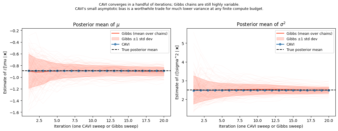

Scaling Up: Stochastic Variational Inference¶

For large datasets the CAVI loop over all $N$ data points can be expensive. Stochastic Variational Inference (SVI) Hoffman et al., 2013 replaces the full-data update with a mini-batch estimate:

Sample a mini-batch $\mathcal{B} \subset \{1,\ldots,N\}$ .
Compute local updates (responsibilities) on the mini-batch.
Scale up the sufficient statistics: $\hat{N}_k = \frac{N}{|\mathcal{B}|} \sum_{n \in \mathcal{B}} \tilde{\omega}_{n,k}$ .
Take a natural gradient step on the global parameters.

SVI can be interpreted as stochastic gradient ascent on the ELBO using the natural gradient Amari, 1998 — the gradient preconditioned by the Fisher information matrix of the variational family.

For exponential-family variational posteriors, the natural gradient update coincides exactly with the CAVI update applied to the mini-batch, making SVI easy to implement.

Conclusion¶

CAVI turns posterior inference into optimisation, providing full variational posteriors over both parameters and latent variables.

Aspect	EM	CAVI
Parameters $\{\mbmu_k, \mbpi\}$	Point estimates	Full posterior $q(\mbmu_k), q(\mbpi)$
Latent variables $\{z_n\}$	Exact posterior	Approximate posterior $q(z_n)$
Objective	Marginal LL	ELBO
Convergence	Monotone ↑ marginal LL	Monotone ↑ ELBO

Key takeaways:

Mean-field CAVI treats each variable as independent under the variational posterior; dependencies are captured only through the updates.
The CAVI update for each factor is $q^\star(\theta_j) \propto \exp\{\mathbb{E}_{q_{\neg j}}[\log p(\theta_j \mid \mbtheta_{\neg j}, \mbx)]\}$ — the exponentiated expected log conditional.
For conjugate exponential-family models, CAVI updates are closed form: the optimal factor has the same form as the prior with updated natural parameters.
The digamma correction in the $q(z_n)$ update replaces $\log \pi_k$ with $\mathbb{E}_q[\log \pi_k] = \psi(\tilde{\alpha}_k) - \psi(\sum_j \tilde{\alpha}_j)$ , propagating uncertainty about $\mbpi$ .
SVI scales CAVI to large datasets via natural gradient mini-batch updates.

Coordinate Ascent Variational Inference

Motivation: Why Variational Inference?¶

The Variational Inference Framework¶

Notation¶

Objective: KL Divergence¶

The Mean-Field Family¶

The CAVI Update¶

CAVI for Gaussian Mixture Models¶

Variational Family¶

Update for q(zn)q(z_n)q(zn​): Responsibilities¶

Update for q(π)q(\mbpi)q(π): Dirichlet¶

Update for q(μk)q(\mbmu_k)q(μk​): Gaussian¶

The ELBO for the Gaussian Mixture Model¶

Demo: CAVI versus MCMC for a Gaussian Model¶

Scaling Up: Stochastic Variational Inference¶

Conclusion¶

Update for $q(z_n)$ : Responsibilities¶

Update for $q(\mbpi)$ : Dirichlet¶

Update for $q(\mbmu_k)$ : Gaussian¶