Gradient-Based VI

CAVI is powerful but requires the variational family to match the conjugate structure of the model. For non-conjugate models — Bayesian logistic regression, neural-network priors, physics-based simulators — no closed-form coordinate updates exist.

Gradient-based variational inference removes the conjugacy requirement by estimating the ELBO gradient with Monte Carlo and optimising with stochastic gradient ascent. This approach goes under several names: black-box VI (BBVI), automatic differentiation VI (ADVI), and fixed-form VI.

The central challenge is differentiating through an expectation:

\nabla_{\mblambda} \mathcal{L}(\mblambda) = \nabla_{\mblambda} \mathbb{E}_{q(\mbtheta;\,\mblambda)} \bigl[\log p(\mbx, \mbtheta) - \log q(\mbtheta; \mblambda)\bigr].

(1)

This chapter covers two gradient estimators that handle this:

Score function estimator (REINFORCE) — broadly applicable but high variance.
Pathwise gradient estimator (reparameterization trick) — lower variance, works whenever we can write $\mbtheta = r(\mblambda, \mbepsilon)$ with $\mbepsilon$ independent of $\mblambda$ .

We conclude with a worked example: ADVI for Bayesian logistic regression, a non-conjugate model where CAVI has no closed-form updates.

Setup¶

Let $\mbtheta$ denote all latent variables and parameters, and let $\mathcal{Q} = \{q(\mbtheta; \mblambda) : \mblambda \in \Lambda\}$ be the variational family. We maximise the ELBO:

\mathcal{L}(\mblambda) = \mathbb{E}_{q(\mbtheta;\,\mblambda)}\!\left[ \log p(\mbx, \mbtheta) - \log q(\mbtheta; \mblambda) \right] = \log p(\mbx) - D_{\mathrm{KL}}\bigl(q(\mbtheta;\mblambda) \| p(\mbtheta \mid \mbx)\bigr).

(2)

Strategy: assume $\Lambda = \mathbb{R}^P$ (unconstrained parameters) and run (stochastic) gradient ascent:

\mblambda \leftarrow \mblambda + \alpha_t\, \widehat{\nabla}_{\mblambda} \mathcal{L}(\mblambda),

(3)

where $\widehat{\nabla}_{\mblambda} \mathcal{L}$ is an unbiased Monte Carlo estimate of the gradient.

The obstacle: the distribution under the expectation depends on $\mblambda$ , so we cannot simply move $\nabla_{\mblambda}$ inside the expectation.

The Score Function Estimator (REINFORCE)¶

Derivation¶

Use the log-derivative trick $\nabla_{\mblambda} q = q \cdot \nabla_{\mblambda} \log q$ to move the gradient inside the integral:

\nabla_{\mblambda} \mathbb{E}_{q(\mbtheta;\,\mblambda)}[h(\mbtheta)] = \int \nabla_{\mblambda} q(\mbtheta; \mblambda) \cdot h(\mbtheta)\,d\mbtheta = \mathbb{E}_{q}\!\left[\underbrace{\nabla_{\mblambda} \log q(\mbtheta; \mblambda)}_{\text{score}}\cdot h(\mbtheta)\right].

(4)

This gives the score function estimator (a.k.a. REINFORCE Williams, 1992):

\widehat{\nabla}_{\mblambda}\mathcal{L}(\mblambda) = \frac{1}{M}\sum_{m=1}^M \Bigl[\nabla_{\mblambda}\log q(\mbtheta^{(m)};\mblambda)\Bigr] \bigl[\log p(\mbx,\mbtheta^{(m)}) - \log q(\mbtheta^{(m)};\mblambda)\bigr], \quad \mbtheta^{(m)} \overset{\text{iid}}{\sim} q(\mbtheta;\mblambda).

(5)

Properties:

Works for discrete and continuous $\mbtheta$ — only requires that $\log q$ is differentiable wrt $\mblambda$ .
Often has high variance in practice.

Variance Reduction: Control Variates¶

Since the score has zero expectation, $\mathbb{E}_q[\nabla_{\mblambda} \log q(\mbtheta; \mblambda)] = 0$ , we can subtract any baseline $b$ without changing the expectation:

\nabla_{\mblambda}\mathcal{L} = \mathbb{E}_q\!\bigl[(h(\mbtheta) - b)\,\nabla_{\mblambda}\log q(\mbtheta;\mblambda)\bigr].

(6)

Choosing $b = \mathbb{E}_q[h(\mbtheta)]$ (the running mean of $h$ ) can reduce variance substantially.

The Pathwise Gradient Estimator (Reparameterisation Trick)¶

Derivation¶

If we can write $\mbtheta = r(\mblambda, \mbepsilon)$ where $\mbepsilon$ has a distribution independent of $\mblambda$ (a reparameterisation), then:

\mathbb{E}_{q(\mbtheta;\,\mblambda)}[h(\mbtheta, \mblambda)] = \mathbb{E}_{\mbepsilon \sim p(\mbepsilon)}[h(r(\mblambda, \mbepsilon), \mblambda)].

(7)

The gradient now passes through the expectation cleanly:

\nabla_{\mblambda} \mathbb{E}_{q}[h(\mbtheta, \mblambda)] = \mathbb{E}_{\mbepsilon}\!\left[\nabla_{\mblambda} h(r(\mblambda, \mbepsilon), \mblambda)\right].

(8)

Monte Carlo estimate:

\widehat{\nabla}_{\mblambda}\mathcal{L}(\mblambda) = \frac{1}{M}\sum_{m=1}^M \nabla_{\mblambda}\bigl[\log p(\mbx, r(\mblambda, \mbepsilon_m)) - \log q(r(\mblambda, \mbepsilon_m); \mblambda)\bigr], \quad \mbepsilon_m \overset{\text{iid}}{\sim} p(\mbepsilon).

(9)

In practice: just call .backward() on a Monte Carlo ELBO estimate computed with reparameterised samples; PyTorch handles the chain rule automatically.

Example: Diagonal Gaussian¶

For $q(\mbtheta; \mbmu, \mbsigma) = \mathcal{N}(\mbtheta; \mbmu, \mathrm{diag}(\mbsigma^2))$ :

\mbtheta = r(\mbmu, \mbsigma, \mbepsilon) = \mbmu + \mbsigma \odot \mbepsilon, \qquad \mbepsilon \sim \mathcal{N}(\mathbf{0}, \mathbf{I}).

(10)

Non-reparameterisable families: Discrete distributions (Bernoulli, Categorical) cannot be reparameterised in the standard sense. For these, the score function estimator (or straight-through / Gumbel-softmax approximations) must be used.

# ── Variance comparison: score function vs pathwise estimator ─────────────
# Model: observe x=5 from N(theta, 1) with prior N(0, 10^2)
# True posterior: N(mu_post, sigma_post^2) by Bayes rule
# Variational: q(theta; mu, log_sigma) = N(mu, sigma^2)

x_obs    = torch.tensor(5.0)
prior_mu, prior_sig = torch.tensor(0.0), torch.tensor(10.0)
lik_sig  = torch.tensor(1.0)

# True posterior  (Gaussian conjugate)
sigma_post = 1.0 / (1/lik_sig**2 + 1/prior_sig**2).sqrt()
mu_post    = sigma_post**2 * (x_obs/lik_sig**2 + prior_mu/prior_sig**2)
print(f'True posterior: N({mu_post.item():.3f}, {sigma_post.item():.3f}²)')

def log_joint(theta):
    return (dist.Normal(theta, lik_sig).log_prob(x_obs)
            + dist.Normal(prior_mu, prior_sig).log_prob(theta))

def elbo_and_grads(mu, log_sigma, M, estimator='pathwise'):
    sigma = log_sigma.exp()
    if estimator == 'pathwise':
        # Reparameterise: theta = mu + sigma * eps
        eps   = torch.randn(M)
        theta = mu + sigma * eps
        lp    = log_joint(theta)
        lq    = dist.Normal(mu, sigma).log_prob(theta)
        elbo  = (lp - lq).mean()
        elbo.backward()
        g_mu, g_ls = mu.grad.clone(), log_sigma.grad.clone()
    else:  # score function
        with torch.no_grad():
            theta = dist.Normal(mu, sigma).rsample((M,))
            lp    = log_joint(theta)
            lq    = dist.Normal(mu, sigma).log_prob(theta)
            h     = lp - lq                             # (M,)
            # score wrt mu: (theta - mu) / sigma^2
            score_mu = (theta - mu) / sigma**2
            # score wrt log_sigma: (theta-mu)^2/sigma^2 - 1
            score_ls = (theta - mu)**2 / sigma**2 - 1.0
            g_mu  = (h * score_mu).mean()
            g_ls  = (h * score_ls).mean()
            elbo  = h.mean()
    return elbo.detach(), g_mu, g_ls

# Measure gradient variance at the true posterior parameters
torch.manual_seed(42)
mu_val, ls_val = mu_post.item(), sigma_post.log().item()
M_vals = [1, 4, 16, 64, 256]

results = {'pathwise': {}, 'score': {}}
n_trials = 500
for M in M_vals:
    for est in ('pathwise', 'score'):
        grads = []
        for _ in range(n_trials):
            mu       = torch.tensor(mu_val, requires_grad=True)
            log_sig  = torch.tensor(ls_val, requires_grad=True)
            _, g, _  = elbo_and_grads(mu, log_sig, M, estimator=est)
            grads.append(g.item())
        results[est][M] = torch.tensor(grads).std().item()

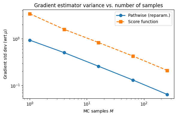
print('\nGradient std (wrt μ) vs. number of MC samples M:')
print(f'  {"M":>6}  {"Pathwise":>12}  {"Score fn":>12}')
for M in M_vals:
    print(f'  {M:>6}  {results["pathwise"][M]:>12.4f}  {results["score"][M]:>12.4f}')

True posterior: N(4.950, 0.995²)


Gradient std (wrt μ) vs. number of MC samples M:
       M      Pathwise      Score fn
       1        0.9316        3.4249
       4        0.5053        1.5912
      16        0.2589        0.8320
      64        0.1316        0.4282
     256        0.0647        0.2110

fig, ax = plt.subplots(figsize=(6, 4))
ax.plot(M_vals, [results['pathwise'][M] for M in M_vals],
        'o-', color=palette[0], lw=2, ms=7, label='Pathwise (reparam.)')
ax.plot(M_vals, [results['score'][M]    for M in M_vals],
        's--', color=palette[1], lw=2, ms=7, label='Score function')
ax.set_xscale('log'); ax.set_yscale('log')
ax.set_xlabel('MC samples $M$')
ax.set_ylabel('Gradient std dev (wrt $\mu$)')
ax.set_title('Gradient estimator variance vs. number of samples')
ax.legend()
plt.tight_layout()

<>:8: SyntaxWarning: invalid escape sequence '\m'
<>:8: SyntaxWarning: invalid escape sequence '\m'
/tmp/ipykernel_2659/3636087577.py:8: SyntaxWarning: invalid escape sequence '\m'
  ax.set_ylabel('Gradient std dev (wrt $\mu$)')

ADVI for Bayesian Logistic Regression¶

Model¶

Consider $N$ binary observations $y_n \in \{0,1\}$ with $D$ -dimensional features $\mbx_n$ . A logistic regression model with Gaussian prior is:

\mbw \sim \mathcal{N}(\mathbf{0}, \tau^2 \mathbf{I}), \qquad y_n \mid \mbw, \mbx_n \sim \operatorname{Bernoulli}\!\bigl(\sigma(\mbw^\top \mbx_n)\bigr),

(11)

where $\sigma(a) = 1/(1+e^{-a})$ is the sigmoid. The posterior $p(\mbw \mid \mbX, \mby)$ has no closed form (the likelihood is not conjugate to the Gaussian prior), making CAVI inapplicable.

Variational Family¶

Use a mean-field Gaussian:

q(\mbw; \mbmu, \boldsymbol{\rho}) = \mathcal{N}\!\bigl(\mbw;\; \mbmu,\; \operatorname{diag}(e^{2\boldsymbol{\rho}})\bigr),

(12)

where $\mbmu, \boldsymbol{\rho} \in \mathbb{R}^D$ are unconstrained variational parameters ( $\mbsigma = e^{\boldsymbol{\rho}}$ enforces positivity).

ELBO¶

\mathcal{L}(\mbmu, \boldsymbol{\rho}) = \underbrace{\mathbb{E}_{q}\!\left[\sum_{n=1}^N \log \sigma(y_n' \mbw^\top \mbx_n)\right]}_{\text{expected log-likelihood (MC)}} - \underbrace{D_{\mathrm{KL}}\!\bigl(\mathcal{N}(\mbmu, \operatorname{diag}(e^{2\boldsymbol{\rho}})) \| \mathcal{N}(\mathbf{0}, \tau^2 \mathbf{I})\bigr)}_{\text{closed form}},

(13)

where $y_n' = 2y_n - 1 \in \{-1, +1\}$ . We estimate the expected log-likelihood via a single reparameterised sample ( $M=1$ ) per gradient step, relying on Adam to average out the noise.

torch.manual_seed(305)

# ── Synthetic binary classification data ─────────────────────────────────────
N, D = 200, 4
w_true = torch.tensor([2.0, -1.5, 0.5, -0.8])
X = torch.randn(N, D)
y = dist.Bernoulli(logits=X @ w_true).sample()
print(f'Data: N={N}, D={D}, fraction positive = {y.mean():.2f}')

# ── ADVI with pathwise gradient estimator (Adam) ──────────────────────────────
def advi_logistic(X, y, τ=2.0, M=1, lr=0.05, num_iters=1000, seed=0):
    """ADVI for Bayesian logistic regression.

    Variational family: q(w) = N(μ, diag(exp(2ρ)))
    Uses the reparameterisation trick + PyTorch autograd.

    Parameters
    ----------
    τ   : prior standard deviation
    M   : MC samples per gradient step
    """
    torch.manual_seed(seed)
    N, D = X.shape

    μ = torch.zeros(D, requires_grad=True)
    ρ = torch.full((D,), -1.0, requires_grad=True)   # log σ, init σ ≈ 0.37

    optimiser = torch.optim.Adam([μ, ρ], lr=lr)
    elbos = []

    for _ in range(num_iters):
        optimiser.zero_grad()

        σ   = ρ.exp()                                # (D,)

        # Reparameterised samples: w = μ + σ * ε,  ε ~ N(0,I)
        ε   = torch.randn(M, D)
        w   = μ.unsqueeze(0) + σ.unsqueeze(0) * ε   # (M, D)

        # Expected log-likelihood  (averaged over M samples and N data points)
        logits   = X @ w.T                           # (N, M)
        log_lik  = dist.Bernoulli(logits=logits).log_prob(y.unsqueeze(1))
        ell      = log_lik.sum(0).mean()             # scalar

        # KL[ N(μ, diag(σ²)) || N(0, τ²I) ] — closed form
        kl = dist.kl_divergence(
            dist.Normal(μ, σ),
            dist.Normal(torch.zeros(D), τ * torch.ones(D))
        ).sum()

        loss = -(ell - kl)                           # minimise negative ELBO
        loss.backward()
        optimiser.step()

        elbos.append(-loss.item())

    return μ.detach(), ρ.exp().detach(), elbos


μ_vi, σ_vi, elbos = advi_logistic(X, y, τ=2.0, M=1, lr=0.05, num_iters=1000)

print('\nADVI posterior means vs. true weights:')
for d in range(D):
    print(f'  w[{d}]: true={w_true[d]:+.2f},  μ_q={μ_vi[d]:+.4f},  σ_q={σ_vi[d]:.4f}')

Data: N=200, D=4, fraction positive = 0.53


ADVI posterior means vs. true weights:
  w[0]: true=+2.00,  μ_q=+2.2546,  σ_q=0.2031
  w[1]: true=-1.50,  μ_q=-2.0509,  σ_q=0.2665
  w[2]: true=+0.50,  μ_q=+0.6147,  σ_q=0.2051
  w[3]: true=-0.80,  μ_q=-0.5289,  σ_q=0.2159

fig, axes = plt.subplots(1, 3, figsize=(13, 4))

# ── Panel 1: ELBO convergence ────────────────────────────────────────────────
axes[0].plot(elbos, lw=1.5, color='steelblue', alpha=0.8)
axes[0].set_xlabel('Iteration')
axes[0].set_ylabel('ELBO')
axes[0].set_title('ADVI: ELBO convergence')

# ── Panel 2: Variational posteriors vs true weights ──────────────────────────
ax = axes[1]
θ_grid = torch.linspace(-4, 4, 300)
for d in range(D):
    q_d = dist.Normal(μ_vi[d], σ_vi[d])
    ax.plot(θ_grid.numpy(), q_d.log_prob(θ_grid).exp().numpy(),
            color=palette[d], lw=2, label=f'$q(w_{d+1})$')
    ax.axvline(w_true[d].item(), color=palette[d], lw=1.5, ls='--', alpha=0.7)
ax.set_xlabel(r'$w$')
ax.set_ylabel('Density')
ax.set_title('Variational posteriors $q(w_d)$\n(dashed = true values)')
ax.legend(fontsize=8)

# ── Panel 3: Predictive accuracy ─────────────────────────────────────────────
ax = axes[2]
# Predict using posterior mean
logits_train = X @ μ_vi
y_pred       = (logits_train > 0).float()
acc_vi       = (y_pred == y).float().mean().item()
# Compare to MLE / MAP
w_mle = torch.linalg.lstsq(X, y.float()).solution
y_pred_mle = ((X @ w_mle) > 0.5).float()
acc_mle = (y_pred_mle == y).float().mean().item()

# MC predictive
M_pred = 1000
ε_pred = torch.randn(M_pred, D)
w_samp = μ_vi.unsqueeze(0) + σ_vi.unsqueeze(0) * ε_pred  # (M_pred, D)
prob_pred = dist.Bernoulli(logits=X @ w_samp.T).probs.mean(1).numpy()

ax.hist(prob_pred[y == 1], bins=20, alpha=0.6, color=palette[0], label='True y=1')
ax.hist(prob_pred[y == 0], bins=20, alpha=0.6, color=palette[1], label='True y=0')
ax.set_xlabel('MC predictive probability $p(y=1 | x_n)$')
ax.set_ylabel('Count')
ax.set_title(f'MC predictive probabilities\n(train accuracy: {acc_vi:.2f})')
ax.legend(fontsize=9)

plt.tight_layout()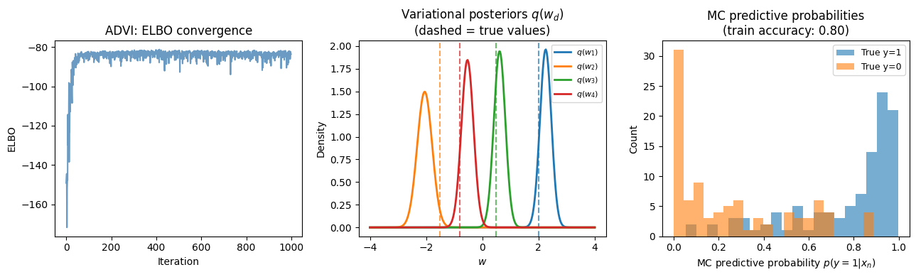

Mini-Batches and Stochastic Optimisers¶

Mini-Batch ELBO¶

When $N$ is large, each gradient step over the full dataset is expensive. We can subsample a mini-batch $\mathcal{B} \subset \{1,\ldots,N\}$ and scale up the log-likelihood:

\mathcal{L}(\mblambda) = \frac{N}{|\mathcal{B}|}\sum_{n \in \mathcal{B}} \mathbb{E}_{q}[\log p(x_n \mid \mbtheta)] - D_{\mathrm{KL}}(q \| p),

(14)

giving an unbiased estimate of the ELBO and its gradient.

Stochastic Optimisers¶

Basic SGD often converges slowly. Several adaptive-step methods work well for ELBO optimisation:

Method	Update rule	Notes
SGD Robbins & Siegmund, 1971	$\mblambda \leftarrow \mblambda + \alpha \hat{g}$	Simple; needs careful $\alpha$ schedule
AdaGrad Duchi et al., 2011	Per-parameter $\alpha / \sqrt{\sum \hat{g}^2}$	Good for sparse gradients
Adam Kingma & Ba, 2014	Momentum + adaptive scale	Default choice; robust

Robbins-Monro conditions for SGD convergence: the step sizes must satisfy $\sum_t \alpha_t = \infty$ and $\sum_t \alpha_t^2 < \infty$ .

Adam is the practical default for ADVI — it rarely requires step-size tuning and handles the varying scales of $\mu$ and $\rho$ automatically.

Conclusion¶

Gradient-based VI removes the conjugacy requirement of CAVI, enabling variational inference in any model where the log joint is differentiable.

	Score function	Pathwise (reparam.)
Requires	Differentiable $\log q$ wrt $\mblambda$	Differentiable reparameterisation $r(\mblambda, \mbepsilon)$
Works for discrete $\mbtheta$ ?	Yes	No (without approximation)
Variance	High	Low
Implementation	Manual score computation	Automatic (`.backward()`)

Key takeaways:

The log-derivative trick converts $\nabla_{\mblambda} \mathbb{E}_q[h]$ into an expectation computable by MC — but with high variance.
The reparameterisation trick decouples sampling noise from $\mblambda$ , moving the gradient inside the expectation and drastically reducing variance.
In PyTorch, reparameterised VI is nearly automatic: construct the ELBO using .rsample(), call .backward(), step an optimiser.
Adam is the practical default; a single MC sample per step ( $M=1$ ) usually suffices when paired with an adaptive optimiser.
The KL term between two Gaussians (or other conjugate pairs) can be computed analytically, reducing MC noise further.

References¶

Williams, R. J. (1992). Simple statistical gradient-following algorithms for connectionist reinforcement learning. Machine Learning, 8(3), 229–256.
Robbins, H., & Siegmund, D. (1971). A convergence theorem for non negative almost supermartingales and some applications. In Optimizing methods in statistics (pp. 233–257). Elsevier.
Duchi, J., Hazan, E., & Singer, Y. (2011). Adaptive subgradient methods for online learning and stochastic optimization. Journal of Machine Learning Research, 12(7).
Kingma, D. P., & Ba, J. (2014). Adam: A method for stochastic optimization. arXiv Preprint arXiv:1412.6980.
Blei, D. M., Kucukelbir, A., & McAuliffe, J. D. (2017). Variational Inference: A Review for Statisticians. Journal of the American Statistical Association, 112(518), 859–877.
Mohamed, S., Rosca, M., Figurnov, M., & Mnih, A. (2020). Monte Carlo Gradient Estimation in Machine Learning. Journal of Machine Learning Research, 21(132), 1–62.