Reinforcement learning (RL) is the study of how an agent learns to make sequential decisions by interacting with an environment in order to maximize cumulative reward Sutton & Barto, 2018. Unlike supervised learning, RL receives no labeled targets — only scalar feedback signals that may be delayed and sparse. This chapter develops the probabilistic foundations of RL, derives the key policy gradient algorithms, and examines the role of RL in modern language model training.
Source
import torch
import numpy as np
import matplotlib.pyplot as plt
from torch import nn
from torch.distributions import Categorical, Beta
Markov Decision Processes
The standard framework for sequential decision-making is the Markov decision process (MDP), defined by a tuple :
: state space (e.g. positions on a grid, token sequences).
: action space (e.g. moves, next tokens).
: transition distribution — the probability of reaching state from state after taking action .
: reward function — the immediate signal received after taking action in state .
: discount factor — how much future rewards are down-weighted relative to immediate ones.
A policy is a distribution over actions given the current state. Starting from , the agent follows the trajectory
where and reward is collected at each step. The return from time is the discounted sum of future rewards:
The objective is to find a policy that maximizes expected return from the initial state:
where denotes a trajectory sampled under .
Value Functions and the Bellman Equations
Two quantities are central to RL algorithms.
The state-value function measures the expected return when starting in state and following thereafter:
The action-value function conditions on both state and action:
Both satisfy Bellman equations — recursive self-consistency conditions. For the optimal policy , these become the Bellman optimality equations:
The advantage function measures how much better action is than the average under :
When , action is better than average in state under .
Policy Gradient Methods
Policy gradient methods directly parameterize the policy and optimize by gradient ascent. The key result is the policy gradient theorem Sutton & Barto, 2018:
This has an elegant derivation. The probability of a trajectory under is
and since the transition probabilities do not depend on ,
Applying the log-derivative trick then yields the theorem.
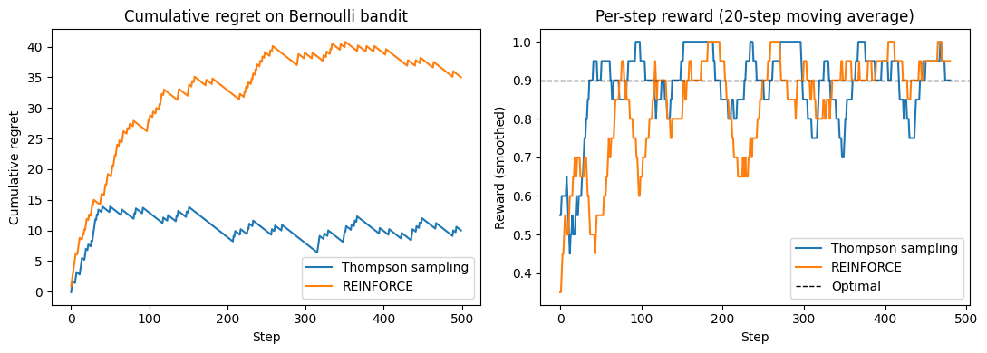
REINFORCE
The simplest policy gradient algorithm is REINFORCE Williams, 1992. Given a batch of trajectories sampled from , the gradient estimate is:
This estimator is unbiased but can have high variance. A common variance-reduction technique subtracts a baseline — typically an estimate of — from the return:
Subtracting the baseline does not introduce bias (it has zero expectation under the policy gradient) but can dramatically reduce variance.
Source
# Multi-armed bandit: compare REINFORCE with Thompson sampling
# K-armed Bernoulli bandit

torch.manual_seed(42)
np.random.seed(42)

K = 5  # number of arms
true_probs = torch.tensor([0.1, 0.3, 0.5, 0.7, 0.9])  # true reward probs
T = 500  # time horizon

# ── Thompson sampling (Bayesian baseline) ──────────────────────────────────────
def thompson_sampling(K, true_probs, T):
    '''Beta-Bernoulli Thompson sampling on a K-armed bandit.'''
    alpha = torch.ones(K)  # Beta(alpha, beta) prior
    beta  = torch.ones(K)
    rewards = []
    for _ in range(T):
        # Sample from posterior
        theta = torch.distributions.Beta(alpha, beta).sample()
        arm = theta.argmax().item()
        reward = (torch.rand(1).item() < true_probs[arm].item())
        rewards.append(float(reward))
        if reward:
            alpha[arm] += 1
        else:
            beta[arm] += 1
    return rewards

# ── REINFORCE on bandit (stateless MDP, one step per episode) ──────────────────
def reinforce_bandit(K, true_probs, T, lr=0.05):
    '''REINFORCE for K-armed bandit: softmax policy, baseline = running mean.'''
    logits = torch.zeros(K, requires_grad=True)
    optimizer = torch.optim.Adam([logits], lr=lr)
    rewards = []
    baseline = 0.0
    alpha_ema = 0.05  # EMA coefficient for baseline
    for t in range(T):
        dist = Categorical(logits=logits)
        arm = dist.sample()
        reward = float(torch.rand(1).item() < true_probs[arm].item())
        rewards.append(reward)
        baseline = (1 - alpha_ema) * baseline + alpha_ema * reward
        loss = -dist.log_prob(arm) * (reward - baseline)
        optimizer.zero_grad()
        loss.backward()
        optimizer.step()
    return rewards

def running_mean(x, w=20):
    return np.convolve(x, np.ones(w)/w, mode='valid')

ts_rewards    = thompson_sampling(K, true_probs, T)
rf_rewards    = reinforce_bandit(K, true_probs, T)

fig, axes = plt.subplots(1, 2, figsize=(11, 4))

# Left: cumulative regret
optimal = true_probs.max().item()
ts_regret = np.cumsum(optimal - np.array(ts_rewards))
rf_regret = np.cumsum(optimal - np.array(rf_rewards))
axes[0].plot(ts_regret, label='Thompson sampling', color='tab:blue')
axes[0].plot(rf_regret, label='REINFORCE', color='tab:orange')
axes[0].set_xlabel('Step'); axes[0].set_ylabel('Cumulative regret')
axes[0].set_title('Cumulative regret on Bernoulli bandit')
axes[0].legend()

# Right: smoothed per-step reward
axes[1].plot(running_mean(ts_rewards), label='Thompson sampling', color='tab:blue')
axes[1].plot(running_mean(rf_rewards), label='REINFORCE', color='tab:orange')
axes[1].axhline(optimal, ls='--', color='k', lw=1, label='Optimal')
axes[1].set_xlabel('Step'); axes[1].set_ylabel('Reward (smoothed)')
axes[1].set_title('Per-step reward (20-step moving average)')
axes[1].legend()

plt.tight_layout()
plt.savefig('bandit_rl.png', dpi=100, bbox_inches='tight')
plt.show()
Actor-Critic Methods and PPO
REINFORCE uses the full Monte Carlo return , which is unbiased but high-variance. Actor-critic methods replace with a lower-variance estimate by maintaining a learned critic alongside the actor . The actor is updated using the advantage estimate
which is an empirical version of the Bellman residual (also called the TD error). The critic is updated to minimize .
Proximal Policy Optimization (PPO)
A key practical challenge in policy gradient methods is choosing a step size: too large a step can collapse the policy, and the resulting poor samples make recovery slow. Trust region methods address this by constraining each update to stay close to the current policy.
PPO Schulman et al., 2017 enforces a soft trust region via a clipped surrogate objective. Define the probability ratio
The PPO objective clips this ratio to prevent large updates:
where is a hyperparameter. When the clip prevents the policy from increasing beyond ; when it prevents a decrease below . PPO is simple to implement, stable, and is the dominant algorithm in large-scale RL applications.
Planning as Inference and Maximum Entropy RL
Control as Inference
The probabilistic graphical models we have studied throughout this course suggest a natural reframing of RL: rather than treating reward maximization as an optimization problem, we can treat it as posterior inference in a suitably defined generative model.
Introduce a sequence of binary optimality variables with the likelihood:
where is a temperature parameter (requiring , or equivalently working with exponentiated rewards after a suitable shift). The full generative model over trajectories and optimality variables is:
The RL objective — finding a policy that maximizes expected reward — is equivalent to computing the posterior distribution over trajectories given that all optimality variables are 1:
This is analogous to the smoothing distribution in a hidden Markov model, computed by a backward message-passing algorithm. Define the backward messages:
Taking logarithms and defining the soft value function and soft Q-function , the backward recursion becomes the soft Bellman equations:
The second equation replaces the hard of standard Bellman optimality with a soft-max (log-sum-exp), recovering the hard-max in the limit .
Maximum Entropy RL
The inference perspective has an equivalent variational characterization. Define the maximum entropy RL objective:
where is the policy entropy. The entropy bonus simultaneously:
Encourages exploration: the policy is penalized for being overly deterministic.
Improves robustness: the policy learns to hedge against uncertainty.
Avoids premature commitment: multiple near-optimal strategies are maintained.
The unique optimal policy for is the Boltzmann / softmax policy:
This is a Gibbs distribution over actions, with the soft Q-function playing the role of an energy. As the policy concentrates on the greedy action; as it approaches the uniform distribution.
Connection to KL Regularization
The MaxEnt objective can be written equivalently as a KL minimization. For a reference policy , the KL-regularized objective
has the same Boltzmann-form optimal solution with in place of the uniform distribution:
This is precisely the RLHF objective studied in the next section. The KL penalty to the reference (SFT) language model is the MaxEnt RL entropy bonus, with the entropy measured relative to rather than the uniform distribution. The closed-form optimal RLHF policy derived earlier is the Boltzmann policy of this MaxEnt problem.
Soft Actor-Critic
In practice, Soft Actor-Critic (SAC) implements MaxEnt RL for continuous action spaces by maintaining:
An actor trained to minimize , which simplifies to maximizing .
A critic trained on the soft Bellman residual, using a target network for stability.
An optional automatic entropy tuning step that adjusts to maintain a target entropy .
SAC is the dominant off-policy MaxEnt RL algorithm for continuous control, achieving strong sample efficiency through experience replay and the stabilizing effect of the entropy bonus.
Reinforcement Learning from Human Feedback
The Language Model as a Policy
A language model can be viewed as a policy in an MDP where:
the state is the prompt (and tokens generated so far),
the action is the next token (vocabulary),
the episode ends at an end-of-sequence token, yielding a full response .
The transition dynamics are deterministic (the generated token becomes part of the state), so the stochasticity in the MDP comes entirely from .
Reward Modeling from Human Preferences
Many desirable properties of language model outputs — helpfulness, harmlessness, honesty — are difficult to specify as an explicit reward function. RLHF Christiano et al., 2017 Ouyang et al., 2022 sidesteps this by learning a reward model from human preference data.
Step 1: Collect preference data. Present human annotators with pairs of responses to the same prompt , and ask which is preferred. The Bradley–Terry model for pairwise preferences gives:
where is a learned reward model and is the sigmoid. The reward model is trained by maximum likelihood on the preference dataset :
Step 2: Fine-tune with RL. Using as the reward signal, fine-tune the language model with PPO to maximize expected reward Ziegler et al., 2019. To prevent the policy from straying too far from the supervised fine-tuned (SFT) reference model , a KL penalty is added:
where controls the strength of the KL penalty. The KL term serves two purposes: it prevents reward hacking (exploiting the reward model), and it ensures the language model retains its general capabilities.
The KL-penalized objective has a closed-form optimal solution. Let be the partition function. Then:
This is a tilted or exponentially weighted version of the reference policy — a familiar form from the importance sampling and energy-based model literatures.
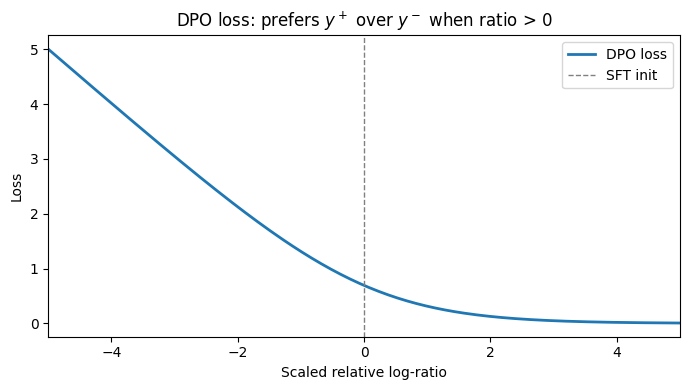
Direct Preference Optimization
Direct Preference Optimization (DPO) Rafailov et al., 2024 observes that, given the closed-form optimal policy above, the reward model can be expressed directly in terms of the language model:
Substituting into the Bradley–Terry preference model and noting that cancels in the difference , the preference probability becomes:
This allows the language model to be trained directly from preference data by maximizing this likelihood — without any separate reward model or RL loop:
DPO is conceptually cleaner and computationally cheaper than PPO-based RLHF, but the two approaches have different empirical trade-offs that remain an active area of research.
Source
# Illustrate the DPO loss as a function of the relative log-ratio.
beta_val = 0.1
delta = torch.linspace(-5, 5, 200)  # beta * (log pi(y+)/pi_ref(y+) - log pi(y-)/pi_ref(y-))

dpo_loss = -torch.log(torch.sigmoid(delta))

fig, ax = plt.subplots(figsize=(7, 4))
ax.plot(delta.numpy(), dpo_loss.numpy(), color='tab:blue', lw=2, label='DPO loss')
ax.axvline(0, ls='--', color='gray', lw=1, label='SFT init')
ax.set_xlabel('Scaled relative log-ratio')
ax.set_ylabel('Loss')
ax.set_title('DPO loss: prefers $y^+$ over $y^-$ when ratio > 0')
ax.legend()
ax.set_xlim(-5, 5)
plt.tight_layout()
plt.savefig('dpo_loss.png', dpi=100, bbox_inches='tight')
plt.show()
Connections and Further Topics
Connections to Probabilistic Inference
The planning-as-inference and maximum entropy RL perspectives developed in the previous section connect RL to the message-passing algorithms (Chapter 14), variational inference (Chapter 10), and energy-based models studied elsewhere in this course. The Boltzmann optimal policy is an exponential family tilting of the reference, familiar from importance sampling and the exponential family posteriors of Chapter 3.
Reward Hacking and Alignment
A central challenge in RLHF is reward hacking: the language model learns to exploit weaknesses in the learned reward model, producing outputs that score highly according to but are not actually preferred by humans. The KL penalty mitigates this, and the optimal trades off reward maximization against staying close to the reference. The DPO derivation makes this trade-off explicit.
Group Relative Policy Optimization (GRPO)
Recent work on reasoning models (e.g. DeepSeek-R1) uses GRPO, a variant that estimates the advantage by comparing multiple sampled responses to the same prompt within a batch, rather than using a learned critic. For a prompt , sample responses and compute:
This avoids training a separate value network while still providing a low-variance baseline for the policy gradient.
Summary
| Algorithm | Key idea | Main use case |
|---|---|---|
| REINFORCE | Monte Carlo policy gradient | Simple environments, language bandit problems |
| Actor-Critic | TD-error advantage, learned critic | Continuous control |
| PPO | Clipped ratio trust region | Large-scale RL, RLHF |
| DPO | Closed-form RL from preferences | Language model alignment |
| GRPO | Group-relative advantage estimate | Reasoning model training |
Conclusion
Reinforcement learning addresses sequential decision-making under uncertainty: an agent interacts with an environment, receives rewards, and must learn a policy that maximizes expected cumulative return. The policy gradient theorem connects the gradient of the expected return to on-policy rollouts, and this insight underlies REINFORCE, actor-critic methods, and the proximal policy optimization (PPO) algorithm used to fine-tune large language models. The planning-as-inference perspective — treating optimal behavior as posterior inference in a graphical model — provides deep connections to variational inference and message passing. Reinforcement learning from human feedback (RLHF) and direct preference optimization (DPO) apply these ideas to align language models with human preferences, casting alignment as a KL-regularized reward maximization problem.
- Sutton, R. S., & Barto, A. G. (2018). Reinforcement Learning: An Introduction (2nd ed.). MIT Press.
- Williams, R. J. (1992). Simple statistical gradient-following algorithms for connectionist reinforcement learning. Machine Learning, 8(3), 229–256.
- Schulman, J., Wolski, F., Dhariwal, P., Radford, A., & Klimov, O. (2017). Proximal policy optimization algorithms. arXiv Preprint arXiv:1707.06347.
- Christiano, P. F., Leike, J., Brown, T., Martic, M., Legg, S., & Amodei, D. (2017). Deep reinforcement learning from human preferences. Advances in Neural Information Processing Systems, 30.
- Ouyang, L., Wu, J., Jiang, X., Almeida, D., Wainwright, C., Mishkin, P., Zhang, C., Agarwal, S., Slama, K., Ray, A., & others. (2022). Training language models to follow instructions with human feedback. Advances in Neural Information Processing Systems, 35, 27730–27744.
- Ziegler, D. M., Stiennon, N., Wu, J., Brown, T. B., Radford, A., Amodei, D., Christiano, P., & Irving, G. (2019). Fine-tuning language models from human preferences. arXiv Preprint arXiv:1909.08593.
- Rafailov, R., Sharma, A., Mitchell, E., Manning, C. D., Ermon, S., & Finn, C. (2024). Direct preference optimization: Your language model is secretly a reward model. Advances in Neural Information Processing Systems, 36.