Exact posterior inference is possible for conjugate models like the ones we studied in the previous chapters. But most interesting models — including the hierarchical Gaussian model with unknown per-school variances — are non-conjugate, and the posterior cannot be computed in closed form.
Markov chain Monte Carlo (MCMC) is the workhorse of Bayesian computation in these settings. Instead of evaluating the posterior analytically, we construct a Markov chain whose stationary distribution is the posterior and then collect samples. Those samples can be used to approximate any posterior expectation.
In this chapter we:
Motivate the Monte Carlo approach to posterior inference
Introduce Markov chains and their key properties (stationarity, detailed balance, ergodicity)
Derive the Metropolis–Hastings algorithm and its Gibbs sampling special case
Implement a Gibbs sampler for the hierarchical Gaussian model from the previous chapter
Assess convergence and efficiency with MCMC diagnostics
Source
import torch
from torch.distributions import Normal, Gamma, TransformedDistribution
from torch.distributions.transforms import PowerTransform
from pyro.ops.stats import effective_sample_size, autocorrelation
import matplotlib.pyplot as plt

class ScaledInvChiSq(TransformedDistribution):
    '''Scaled inverse chi-squared distribution chi^{-2}(nu, sigma^2).

    Implemented as PowerTransform(-1) of Gamma(nu/2, nu*sigma^2/2),
    matching the parameterization from the previous chapter.
    '''
    def __init__(self, ν, σ2):
        super().__init__(Gamma(ν / 2, ν * σ2 / 2), [PowerTransform(-1)])
/opt/hostedtoolcache/Python/3.13.13/x64/lib/python3.13/site-packages/tqdm/auto.py:21: TqdmWarning: IProgress not found. Please update jupyter and ipywidgets. See https://ipywidgets.readthedocs.io/en/stable/user_install.html
from .autonotebook import tqdm as notebook_tqdm
Posterior Expectations
The central object of Bayesian inference is the posterior distribution . In practice we rarely need the full density; instead we interact with it through expectations:
— the posterior mean,
— the posterior probability that lies in set ,
— the posterior predictive density of new data .
All of these have the form for some function .
Quadrature
One numerical approach is quadrature: place a grid over and approximate
where is the volume element around . This works for low-dimensional posteriors (say ), but the number of grid points needed grows as for a desired accuracy , so it quickly becomes infeasible.
Monte Carlo
Monte Carlo replaces the grid with samples:
Letting :
Unbiasedness: .
Variance: if the samples are uncorrelated, , so the RMSE scales as regardless of dimension .
The catch: how do we draw samples from when we cannot even compute the normalizing constant ?
Markov Chain Monte Carlo
Idea: design a Markov chain whose stationary distribution is the posterior. Run it long enough and the chain’s states become approximate draws from .
Markov Chains
A Markov chain is a sequence of random variables with the Markov property: each state depends on the past only through the immediately preceding state,
is the initial distribution and is the (homogeneous) transition kernel.
Stationary Distributions
Let denote the marginal distribution of the -th state. A distribution is a stationary distribution if
Starting from and applying the transition keeps the distribution unchanged.
Detailed Balance
A sufficient condition for to be stationary is detailed balance:
Integrating both sides over recovers the stationarity equation, so detailed balance implies stationarity.
Ergodicity
Detailed balance shows is a stationary distribution, but not necessarily the unique one. A chain is ergodic if regardless of the starting point . For our purposes, ergodicity holds whenever the transition kernel assigns positive probability to any region of from any starting point (i.e., the chain is irreducible and aperiodic).
The Metropolis–Hastings Algorithm
Our goal is to build an ergodic Markov chain with stationary distribution .
Key observation: even though we cannot compute (because is intractable), we can compute ratios of posterior densities, since the normalizing constant cancels:
The Accept–Reject Step
Metropolis–Hastings constructs the transition kernel from two steps:
Propose a new state by sampling from a proposal distribution .
Accept the proposal with probability ; otherwise stay at .
The resulting transition kernel is
Plugging into the detailed balance condition and solving for the acceptance probability gives the Metropolis–Hastings acceptance probability:
When the ratio exceeds 1 the proposal is always accepted; otherwise it is accepted with probability equal to the ratio. Any proposal that covers yields an ergodic chain.
The Metropolis Algorithm
When the proposal is symmetric (), the proposal densities cancel and
This Metropolis algorithm always accepts moves that increase the joint probability and accepts downhill moves with some probability.
Gibbs Sampling
Gibbs sampling is a special case of Metropolis–Hastings that updates one coordinate at a time by sampling from its complete conditional .
The proposal is
i.e., draw a new from its conditional and keep all other coordinates fixed. Substituting into the MH acceptance probability shows that this proposal is always accepted:
Cycling through all coordinates produces an ergodic chain as long as each complete conditional covers the full support.
def gibbs(theta, X, num_samples):
    samples = []
    for _ in range(num_samples):
        for d in range(len(theta)):
            theta[d] = sample_conditional(d, theta, X)
        samples.append(theta.copy())
    return samples
The key requirement is that we can sample each complete conditional. In conjugate models (like the hierarchical Gaussian below), closed-form conditionals make Gibbs extremely efficient. When some conditionals are intractable, we can mix Gibbs and MH updates in the same chain — the Metropolis-Hastings within Gibbs strategy.
Worked Example: Hierarchical Gaussian Model
We return to the “8 Schools” example from the previous chapter, but now place a prior on the per-school variances as well. This makes the model non-conjugate and exact inference intractable.
We derive the complete conditionals for each variable and implement a Gibbs sampler.
# Hyperparameters
S = 8                    # number of schools
Ns = torch.tensor(20)    # students per school
μ0, κ0 = 0.0, 0.1  # prior on μ
ν0, τ2_0 = 0.1, 100.0 # prior on τ²
α0, σ2_0 = 0.1, 10.0  # prior on σ_s²

# Synthetic data: match sample means/stds to the 8 Schools values
torch.manual_seed(305)
x_bars  = torch.tensor([28.,  8., -3.,  7., -1.,  1., 18., 12.])
σ_bars  = torch.tensor([15., 10., 16., 11.,  9., 11., 10., 18.])
xs_raw  = Normal(x_bars, torch.sqrt(Ns.float()) * σ_bars).sample((Ns,))
zs      = (xs_raw - xs_raw.mean(0)) / xs_raw.std(0)
xs      = x_bars + torch.sqrt(Ns.float()) * σ_bars * zs  # shape (Ns, S)
assert torch.allclose(xs.mean(0), x_bars)
assert torch.allclose(xs.std(0),  torch.sqrt(Ns.float()) * σ_bars)
Log Joint Probability
We track during sampling as a convergence diagnostic.
def log_joint(τ2, μ, θs, σ2s, xs, τ2_0, ν0, μ0, κ0, α0, σ2_0):
    lp  = ScaledInvChiSq(ν0, τ2_0).log_prob(τ2)
    lp += Normal(μ0, torch.sqrt(τ2 / κ0)).log_prob(μ)
    lp += Normal(μ,  torch.sqrt(τ2)).log_prob(θs).sum()
    lp += ScaledInvChiSq(α0, σ2_0).log_prob(σ2s).sum()
    lp += Normal(θs, torch.sqrt(σ2s)).log_prob(xs).sum()
    return lp
Complete Conditional for 
Combining the prior with the likelihoods gives
where
Because each depends only on its own school’s data, all can be sampled in parallel as a blocked Gibbs step.
def gibbs_θs(τ2, μ, σ2s, xs):
    Ns = xs.shape[0]
    v_θ   = 1 / (Ns / σ2s + 1 / τ2)
    θ_hat = v_θ * (xs.sum(0) / σ2s + μ / τ2)
    return Normal(θ_hat, torch.sqrt(v_θ)).sample()
Complete Conditional for 
Combining with the residuals gives a conjugate update:
where
All variances are conditionally independent and sampled in parallel.
def gibbs_σ2s(α0, σ2_0, θs, xs):
    Ns  = xs.shape[0]
    αN  = α0 + Ns
    σ2N = (α0 * σ2_0 + torch.sum((xs - θs) ** 2, dim=0)) / αN
return ScaledInvChiSq(αN, σ2N).sample()def gibbs_μ(μ0, κ0, τ2, θs):
S = len(θs)
v_μ = τ2 / (κ0 + S)
μ_hat = (κ0 * μ0 + θs.sum()) / (κ0 + S)
return Normal(μ_hat, torch.sqrt(v_μ)).sample()def gibbs_τ2(ν0, τ2_0, μ0, κ0, μ, θs):
S = len(θs)
νN = ν0 + S + 1
τ2N = (ν0 * τ2_0 + κ0 * (μ - μ0)**2 + torch.sum((θs - μ)**2)) / νN
return ScaledInvChiSq(νN, τ2N).sample()The Gibbs Sampler
Cycle through the four updates, recording the log joint probability at each step.
def gibbs(xs, τ2_0, ν0, μ0, κ0, α0, σ2_0, num_samples=1000):
    Ns, S = xs.shape

    # Initialise from the prior
    τ2  = ScaledInvChiSq(ν0, τ2_0).sample()
    μ   = Normal(μ0, torch.sqrt(τ2 / κ0)).sample()
    θs  = Normal(μ,  torch.sqrt(τ2)).sample((S,))
    σ2s = ScaledInvChiSq(α0, σ2_0).sample((S,))

    records = []
    for _ in range(num_samples):
        τ2  = gibbs_τ2(ν0, τ2_0, μ0, κ0, μ, θs)
        μ   = gibbs_μ(μ0, κ0, τ2, θs)
        θs  = gibbs_θs(τ2, μ, σ2s, xs)
        σ2s = gibbs_σ2s(α0, σ2_0, θs, xs)
        lp  = log_joint(τ2, μ, θs, σ2s, xs,
                       τ2_0, ν0, μ0, κ0, α0, σ2_0)
        records.append((τ2, μ, θs, σ2s, lp))

    keys = ['τ2', 'μ', 'θs', 'σ2s', 'lps']
    return {k: torch.stack(v) for k, v in zip(keys, zip(*records))}
torch.manual_seed(305)
num_samples = 10000
samples = gibbs(xs, τ2_0, ν0, μ0, κ0, α0, σ2_0, num_samples)MCMC Diagnostics
Before trusting the samples, we check that the chain has converged to the stationary distribution and is mixing efficiently.
Burn-in
The first few iterations reflect the arbitrary initial state. We discard this burn-in period before computing estimates.
Source
fig, axs = plt.subplots(1, 2, figsize=(10, 3))

axs[0].plot(samples['lps'].numpy())
axs[0].set_xlabel('Iteration')
axs[0].set_ylabel('Log joint probability')
axs[0].set_title('All iterations')

burnin = 100
axs[1].plot(torch.arange(burnin, num_samples).numpy(),
            samples['lps'][burnin:].numpy())
axs[1].set_xlabel('Iteration')
axs[1].set_title(f'Iterations {burnin}+')

plt.tight_layout()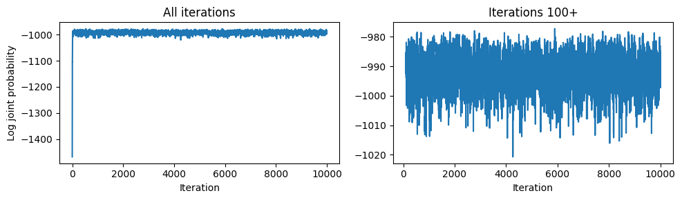
Trace Plots and Marginal Posteriors
After discarding burn-in, we visualize traces and marginal posterior histograms.
Source
fig, axs = plt.subplots(2, 2, figsize=(10, 6))

τ_samp = torch.sqrt(samples['τ2'][burnin:])
axs[0,0].plot(τ_samp.numpy()); axs[0,0].set_ylabel(r'$\tau$'); axs[0,0].set_title('Trace')
axs[0,1].hist(τ_samp.numpy(), 50, density=True, alpha=0.6, ec='k')
axs[0,1].set_xlabel(r'$\tau$'); axs[0,1].set_title(r'Posterior $p(\tau \mid \mathbf{X})$')

μ_samp = samples['μ'][burnin:]
axs[1,0].plot(μ_samp.numpy()); axs[1,0].set_ylabel(r'$\mu$')
axs[1,1].hist(μ_samp.numpy(), 50, density=True, alpha=0.6, ec='k')
axs[1,1].set_xlabel(r'$\mu$'); axs[1,1].set_title(r'Posterior $p(\mu \mid \mathbf{X})$')

plt.tight_layout()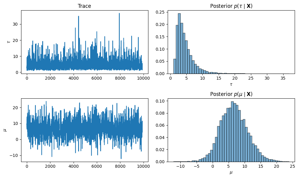
Source
bins = torch.linspace(-30, 30, 80).numpy()
fig, axs = plt.subplots(S, 2, figsize=(10, 10), sharex='col')
for s in range(S):
    axs[s, 0].plot(samples['θs'][burnin:, s].numpy())
    axs[s, 0].set_ylabel(rf'$\theta_{{{s+1}}}$', fontsize=9)
    axs[s, 1].hist(samples['θs'][:, s].numpy(), bins, density=True, alpha=0.6, ec='k')
    axs[s, 1].axvline(xs.mean(0)[s].item(), color='r', lw=1.5,
                      label=r'$\bar{x}_s$' if s == 0 else None)
    axs[s, 1].set_ylabel(rf'$p(\theta_{{{s+1}}}\mid\mathbf{{X}})$', fontsize=8)
axs[0, 0].set_title('Traces'); axs[0, 1].set_title('Posteriors')
axs[0, 1].legend()
axs[-1, 0].set_xlabel('Iteration'); axs[-1, 1].set_xlabel(r'$\theta_s$')
plt.tight_layout()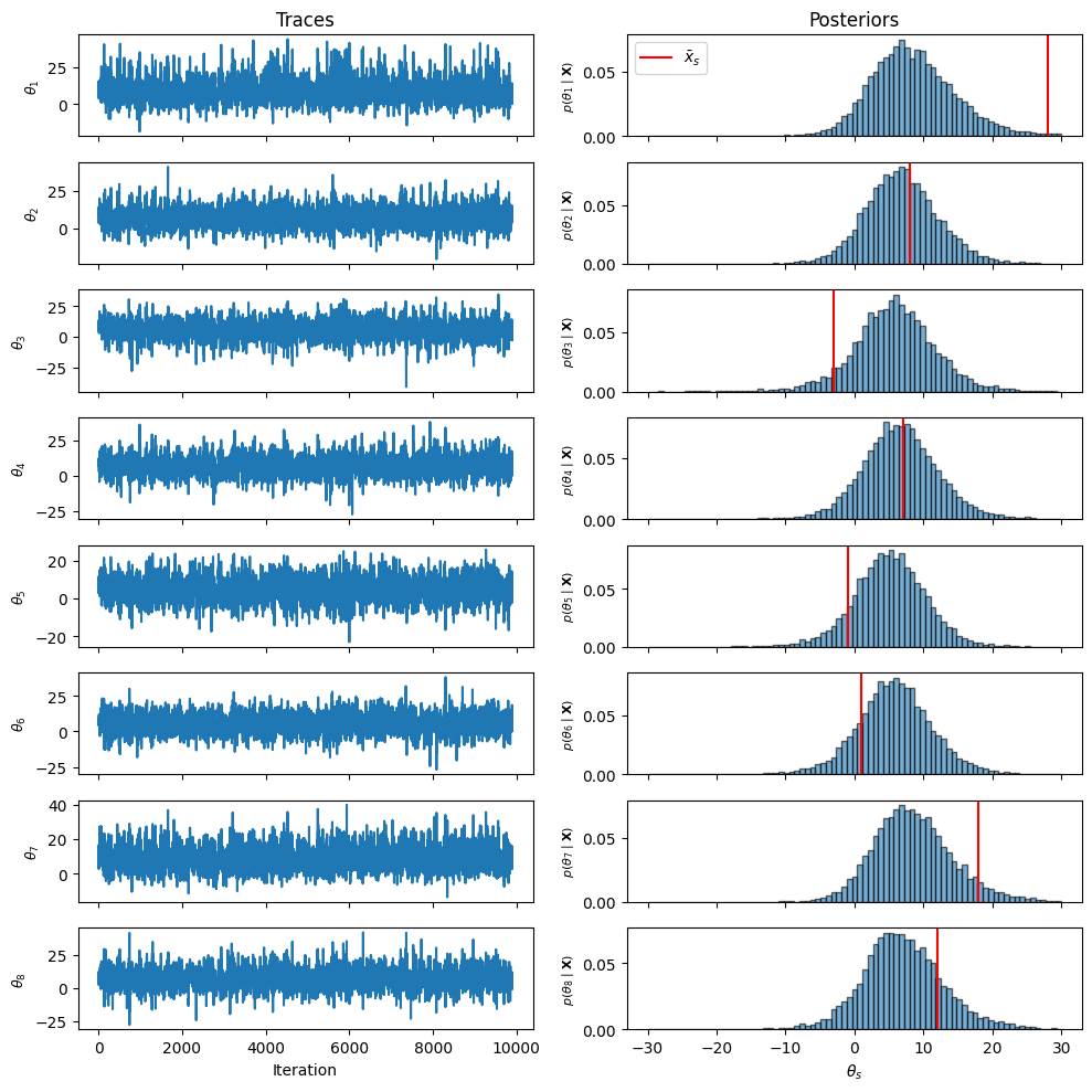
Source
bins = torch.linspace(0, 30, 60).numpy()
σ_samp = torch.sqrt(samples['σ2s'] / Ns.float())  # sigma_bar_s = sigma_s / sqrt(Ns)
fig, axs = plt.subplots(S, 2, figsize=(10, 10), sharex='col')
for s in range(S):
    axs[s, 0].plot(σ_samp[burnin:, s].numpy())
    axs[s, 0].set_ylabel(rf'$\bar{{\sigma}}_{{{s+1}}}$', fontsize=9)
    axs[s, 1].hist(σ_samp[:, s].numpy(), bins, density=True, alpha=0.6, ec='k')
    axs[s, 1].axvline(σ_bars[s].item(), color='r', lw=1.5,
                      label=r'$\bar{\sigma}_s$' if s == 0 else None)
    axs[s, 1].set_ylabel(rf'$p(\bar{{\sigma}}_{{{s+1}}}\mid\mathbf{{X}})$', fontsize=8)
axs[0, 0].set_title('Traces'); axs[0, 1].set_title('Posteriors')
axs[0, 1].legend()
axs[-1, 0].set_xlabel('Iteration'); axs[-1, 1].set_xlabel(r'$\bar{\sigma}_s$')
plt.tight_layout()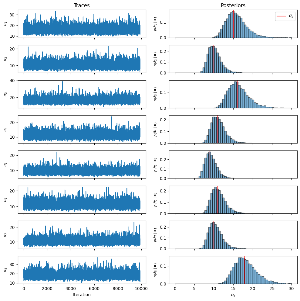
Autocorrelation and Effective Sample Size
Even after burn-in, consecutive MCMC samples are correlated. This inflates the variance of Monte Carlo estimates.
The autocorrelation function at lag is
The effective sample size (ESS) accounts for autocorrelation:
signals slow mixing. For intuition: a random walk with autocorrelation has , which goes to zero as .
Source
acf_τ  = autocorrelation(torch.sqrt(samples['τ2'][burnin:]))
acf_μ  = autocorrelation(samples['μ'][burnin:])
acf_θ1 = autocorrelation(samples['θs'][burnin:, 0])
acf_σ1 = autocorrelation(torch.sqrt(samples['σ2s'])[burnin:, 0])

plt.figure(figsize=(7, 4))
for acf, label in [(acf_τ, r'$\tau$'), (acf_μ, r'$\mu$'),
                   (acf_θ1, r'$\theta_1$'), (acf_σ1, r'$\sigma_1$')]:
    plt.plot(acf[:250].numpy(), label=label)
plt.axhline(0, color='k', lw=0.5)
plt.xlabel('Lag'); plt.ylabel('Autocorrelation'); plt.legend()
plt.tight_layout()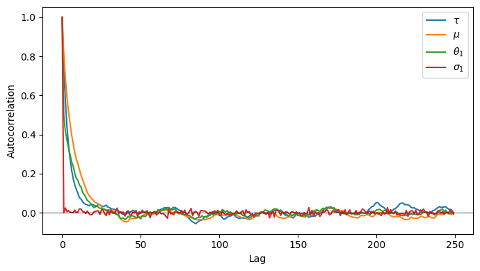
print(f'Effective sample sizes (out of {num_samples - burnin} post-burnin samples):')
print(f"  τ²:   {effective_sample_size(samples['τ2'][None, burnin:]).item():.0f}")
print(f"  μ:    {effective_sample_size(samples['μ'][None, burnin:]).item():.0f}")
print(f"  θ₁:   {effective_sample_size(samples['θs'][None, burnin:, 0]).item():.0f}")
print(f"  σ₁²:  {effective_sample_size(samples['σ2s'][None, burnin:, 0]).item():.0f}")
Effective sample sizes (out of 9900 post-burnin samples):
τ²: 1538
μ: 734
  θ₁:   1113
  σ₁²:  9069
Conclusion
This chapter introduced MCMC as a general-purpose engine for posterior inference and implemented a Gibbs sampler for the hierarchical Gaussian model. Key points:
Posterior expectations are the operative output; Monte Carlo provides a dimension-free approximation.
Metropolis–Hastings constructs a valid transition kernel from any proposal, using only the ratio of joint probabilities (no normalizing constant needed).
Gibbs sampling is MH with exact-conditional proposals that always accept — highly efficient in conjugate or partially-conjugate models.
Blocked Gibbs samples conditionally-independent variables jointly, which is faster and reduces autocorrelation.
Diagnostics — log joint traces, ACF plots, and ESS — are essential for verifying convergence and mixing.
- Bishop, C. M. (2006). Pattern recognition and machine learning. Springer.
- Murphy, K. P. (2023). Probabilistic Machine Learning: Advanced Topics. MIT Press. https://probml.github.io/pml-book/book2.html
- Gelman, A., Carlin, J. B., Stern, H. S., Dunson, D. B., Vehtari, A., & Rubin, D. B. (2013). Bayesian Data Analysis (3rd ed.). Chapman.