Hamiltonian Monte Carlo

Gibbs sampling and random-walk Metropolis–Hastings are powerful, but they scale poorly with dimension. A random-walk proposal explores parameter space by diffusing, which requires $O(D^2)$ steps to produce an independent sample in a $D$ -dimensional space.

Hamiltonian Monte Carlo (HMC) uses gradient information to make large, directed moves through parameter space, reducing that cost to roughly $O(D^{5/4})$ . The key idea is to interpret the negative log-probability as a potential energy surface and simulate the physics of a frictionless particle sliding over it.

In this chapter we:

Motivate gradient-based proposals starting from the Metropolis-Adjusted Langevin Algorithm (MALA)
Derive Hamilton’s equations and their key properties
Implement the leapfrog integrator, the numerical engine of HMC
Assemble the full HMC algorithm and verify it on a 2D correlated Gaussian
Compare HMC against random-walk MH as dimension grows

/opt/hostedtoolcache/Python/3.13.13/x64/lib/python3.13/site-packages/tqdm/auto.py:21: TqdmWarning: IProgress not found. Please update jupyter and ipywidgets. See https://ipywidgets.readthedocs.io/en/stable/user_install.html
  from .autonotebook import tqdm as notebook_tqdm

Why Random Walks Are Slow¶

In Metropolis–Hastings with a symmetric Gaussian proposal $q(\mbtheta' \mid \mbtheta) = \cN(\mbtheta' \mid \mbtheta, \tau^2 \mbI)$ , the chain diffuses through $\Theta$ . To maintain a reasonable acceptance rate, the proposal s.d. $\tau$ must be comparable to the smallest marginal s.d. of the posterior. Each step is then roughly uncorrelated only in that most-constrained direction, while in wider directions many steps are needed to traverse the distribution. The upshot: $O(D^2)$ gradient evaluations to produce one effectively independent sample Neal, 2011.

Metropolis-Adjusted Langevin Algorithm¶

One improvement is to drift the proposal toward high-probability regions using the gradient:

\begin{align} q(\mbtheta' \mid \mbtheta) &= \cN\!\bigl(\mbtheta + \tau \nabla_{\mbtheta} \log p(\mbtheta, \mbX),\; 2\tau^2 \mbI\bigr). \end{align}

(1)

This Metropolis-Adjusted Langevin Algorithm (MALA) is a discrete-time approximation to the Langevin diffusion SDE. It needs only $O(D^{4/3})$ gradient evaluations per independent sample — better than random-walk MH, but we can do better still by taking multiple gradient steps per proposal. That is the idea behind HMC.

Hamiltonian Dynamics¶

Setup¶

Think of the negative log-probability as a potential energy surface. Introduce an auxiliary momentum variable $\mbp \in \reals^D$ (one per parameter) and define the Hamiltonian:

\begin{align} H(\mbq, \mbp) &= U(\mbq) + K(\mbp), \qquad U(\mbq) = -\log p(\mbtheta = \mbq, \mbX), \qquad K(\mbp) = \tfrac{1}{2}\mbp^\top \mbM^{-1} \mbp, \end{align}

(2)

where $\mbM$ is a symmetric positive-definite mass matrix (typically $\mbM = m\mbI$ ).

The joint distribution over position and momentum factorizes:

\begin{align} p(\mbq, \mbp) \propto \exp\{-H(\mbq, \mbp)\} = \underbrace{p(\mbtheta = \mbq \mid \mbX)}_{\text{posterior}} \times \underbrace{\cN(\mbp \mid \mbzero, \mbM)}_{\text{auxiliary}}. \end{align}

(3)

Marginalizing out $\mbp$ recovers the posterior, so samples of $\mbq$ from this joint distribution are posterior samples.

Hamilton’s Equations¶

The state $(\mbq, \mbp)$ evolves in continuous time according to:

\begin{align} \frac{dq_d}{dt} &= \phantom{-}\frac{\partial H}{\partial p_d} = [\mbM^{-1}\mbp]_d, \\ \frac{dp_d}{dt} &= -\frac{\partial H}{\partial q_d} = -\frac{\partial U}{\partial q_d}. \end{align}

(4)

Three key properties of these dynamics make them useful for MCMC:

Reversibility: negating $\mbp$ reverses the trajectory, making the proposal symmetric after a final momentum flip.
Conservation of energy: $\frac{dH}{dt} = 0$ , so the Hamiltonian is constant along trajectories. If the dynamics could be simulated exactly, every HMC proposal would be accepted.
Volume preservation: the divergence of the vector field is zero (since $\frac{\partial^2 H}{\partial q_d \partial p_d} = \frac{\partial^2 H}{\partial p_d \partial q_d}$ ), so Liouville’s theorem applies and there is no Jacobian correction in the acceptance probability.

1D Example: Harmonic Oscillator¶

When $D=1$ , $U(q) = \tfrac{1}{2}q^2$ , and $m=1$ , Hamilton’s equations become $\dot{q} = p$ , $\dot{p} = -q$ — a rotation in $(q, p)$ space. The exact solution is $\mbz(t) = e^{\mbJ t} \mbz(0)$ where $\mbJ = \bigl[\begin{smallmatrix}0&1\\-1&0\end{smallmatrix}\bigr]$ , tracing a circle of constant Hamiltonian.

The Leapfrog Integrator¶

Euler vs. Leapfrog¶

Naïve Euler integration updates position and momentum simultaneously:

\begin{align} \mbp(t+\epsilon) &= \mbp(t) - \epsilon \nabla_{\mbq} U(\mbq(t)), \\ \mbq(t+\epsilon) &= \mbq(t) + \epsilon \mbM^{-1} \mbp(t). \end{align}

(5)

Euler integration does not preserve volume and introduces systematic energy drift even for small $\epsilon$ .

The leapfrog integrator interleaves half-steps for momentum with full steps for position:

\begin{align} \mbp(t + \tfrac{\epsilon}{2}) &= \mbp(t) - \tfrac{\epsilon}{2} \nabla_{\mbq} U(\mbq(t)), \\ \mbq(t + \epsilon) &= \mbq(t) + \epsilon \mbM^{-1} \mbp(t + \tfrac{\epsilon}{2}), \\ \mbp(t + \epsilon) &= \mbp(t + \tfrac{\epsilon}{2}) - \tfrac{\epsilon}{2} \nabla_{\mbq} U(\mbq(t + \epsilon)). \end{align}

(6)

Each update is a shear transformation (only some variables change, by amounts depending on the others), which has unit Jacobian. Composing shears preserves volume exactly. $L$ consecutive leapfrog steps cost $L+1$ gradient evaluations ( $L-1$ full steps sandwiched between two half-steps).

def leapfrog(q, p, grad_U, ε, L, M_inv):
    """Simulate L leapfrog steps of size ε.

    Args:
        q:       (D,) position
        p:       (D,) momentum
        grad_U:  callable, returns gradient of U at q
        ε:       step size
        L:       number of leapfrog steps
        M_inv:   (D, D) inverse mass matrix

    Returns:
        q, p after L steps
    """
    p = p - (ε / 2) * grad_U(q)
    for _ in range(L - 1):
        q = q + ε * (M_inv @ p)
        p = p - ε * grad_U(q)
    q = q + ε * (M_inv @ p)
    p = p - (ε / 2) * grad_U(q)
    return q, p

# Compare Euler and Leapfrog on a 1D harmonic oscillator: U(q)=q²/2, m=1
# Exact solution: (q,p) traces a circle of radius sqrt(q0²+p0²)
grad_U_1d = lambda q: q   # dU/dq = q
M_inv_1d  = torch.eye(1)

q0, p0 = torch.tensor([1.0]), torch.tensor([0.0])
steps  = 30

# Euler
q_e, p_e = q0.clone(), p0.clone()
traj_euler = [(q_e.item(), p_e.item())]
for _ in range(steps):
    p_e = p_e - 0.3 * q_e
    q_e = q_e + 0.3 * p_e
    traj_euler.append((q_e.item(), p_e.item()))

# Leapfrog (each call = 1 leapfrog step)
q_l, p_l = q0.clone(), p0.clone()
traj_leap = [(q_l.item(), p_l.item())]
for _ in range(steps):
    q_l, p_l = leapfrog(q_l, p_l, grad_U_1d, 0.3, 1, M_inv_1d)
    traj_leap.append((q_l.item(), p_l.item()))

# Exact circle
θ_circ = torch.linspace(0, 2 * torch.pi, 200)
q_circ, p_circ = torch.cos(θ_circ).numpy(), torch.sin(θ_circ).numpy()

fig, axs = plt.subplots(1, 2, figsize=(9, 4))
for ax, traj, title in [
    (axs[0], traj_euler, 'Euler (ε = 0.3, 30 steps)'),
    (axs[1], traj_leap,  'Leapfrog (ε = 0.3, 30 steps)')]:
    qs, ps = zip(*traj)
    ax.plot(q_circ, p_circ, 'k--', lw=1, label='exact')
    ax.plot(qs, ps, 'o-', ms=4, label='numerical')
    ax.set_xlabel('q'); ax.set_ylabel('p')
    ax.set_title(title); ax.legend(); ax.set_aspect('equal')
plt.tight_layout()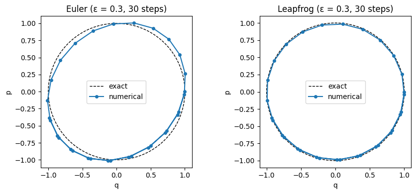

The HMC Algorithm¶

Using Hamiltonian Dynamics as a Proposal¶

HMC is Metropolis–Hastings on the joint distribution $p(\mbq, \mbp)$ with proposals generated by leapfrog integration.

Algorithm (one HMC iteration starting from $\mbq$ ):

Resample momentum: $\mbp \sim \cN(\mbzero, \mbM)$ .
Leapfrog $L$ steps: integrate Hamilton’s equations for time $L\epsilon$ to obtain proposed $(\mbq^*, \mbp^*)$ .
Flip momentum: $\mbp^* \leftarrow -\mbp^*$ (makes the proposal symmetric).
Accept/reject:

\begin{align} a = \min\!\left\{1,\; \exp\bigl(H(\mbq, \mbp) - H(\mbq^*, \mbp^*)\bigr) \right\}. \end{align}

(7)

If $H$ were exactly conserved (exact dynamics), $a = 1$ always. In practice the leapfrog introduces $O(\epsilon^2)$ energy error, so some rejections occur, and a smaller $\epsilon$ gives a higher acceptance rate at the cost of smaller steps.

Tuning¶

The two hyperparameters are the step size $\epsilon$ and the number of steps $L$ :

$\epsilon$ controls accuracy: smaller $\epsilon$ → higher acceptance rate but smaller moves.
$L$ controls how far each proposal travels: larger $L$ → more decorrelated samples but more gradient evaluations per step.

A target acceptance rate of ~0.65 is commonly used for step-size adaptation. The No-U-Turn Sampler (NUTS; Hoffman & Gelman, 2014) automatically adapts $L$ by continuing the trajectory until it starts turning back on itself — eliminating the need to tune $L$ by hand. NUTS is the default sampler in Stan and Pyro.

def hmc(q0, log_joint, grad_U, ε, L, M, num_samples):
    """Hamiltonian Monte Carlo sampler.

    Args:
        q0:          (D,) initial position
        log_joint:   callable: q -> scalar log p(q, X)
        grad_U:      callable: q -> (D,) gradient of -log_joint
        ε:           leapfrog step size
        L:           number of leapfrog steps per proposal
        M:           (D, D) mass matrix
        num_samples: number of HMC iterations

    Returns:
        (num_samples+1, D) tensor of samples (including q0),
        acceptance rate
    """
    M_inv  = torch.linalg.inv(M)
    M_chol = torch.linalg.cholesky(M)
    q       = q0.clone()
    samples = [q.clone()]
    n_accept = 0

    for _ in range(num_samples):
        p = M_chol @ torch.randn_like(q)
        H_curr = -log_joint(q) + 0.5 * p @ M_inv @ p

        q_prop, p_prop = leapfrog(q.clone(), p.clone(), grad_U, ε, L, M_inv)
        H_prop = -log_joint(q_prop) + 0.5 * p_prop @ M_inv @ p_prop

        if torch.rand(1).item() < torch.exp(H_curr - H_prop).item():
            q = q_prop
            n_accept += 1
        samples.append(q.clone())

    return torch.stack(samples), n_accept / num_samples

Demo: 2D Correlated Gaussian¶

We test HMC on a correlated bivariate Gaussian with $\rho = 0.95$ , whose contours form elongated ellipses. This is a hard case for random-walk MH: the optimal proposal must be tiny in the narrow direction, causing slow exploration of the wide direction.

torch.manual_seed(305)

# 2D correlated Gaussian: Σ with off-diagonal ρ
ρ   = 0.95
Σ   = torch.tensor([[1.0, ρ], [ρ, 1.0]])
Σ_inv = torch.linalg.inv(Σ)

def log_joint_2d(q):
    return -0.5 * q @ Σ_inv @ q

def grad_U_2d(q):
    return Σ_inv @ q    # gradient of U = -log_joint

# Run HMC
M_2d  = torch.eye(2)
q0_2d = torch.zeros(2)
samples_hmc, acc_hmc = hmc(q0_2d, log_joint_2d, grad_U_2d,
                            ε=0.2, L=20, M=M_2d, num_samples=2000)
print(f'HMC acceptance rate: {acc_hmc:.2f}')

HMC acceptance rate: 0.99

# Draw one HMC trajectory to illustrate the leapfrog path
torch.manual_seed(1)
q_demo = torch.tensor([-1.5, 1.0])
p_demo = M_2d @ torch.randn(2)
traj_q = [q_demo.clone()]
q_t, p_t = q_demo.clone(), p_demo.clone()
M_inv_2d = torch.linalg.inv(M_2d)
for _ in range(20):
    q_t, p_t = leapfrog(q_t, p_t, grad_U_2d, 0.2, 1, M_inv_2d)
    traj_q.append(q_t.clone())
traj_q = torch.stack(traj_q)

# Contour grid
g = torch.linspace(-3, 3, 200)
Q1, Q2 = torch.meshgrid(g, g, indexing='ij')
Z_grid = torch.stack([Q1.flatten(), Q2.flatten()], dim=1)
log_p  = (-0.5 * (Z_grid @ Σ_inv * Z_grid).sum(1)).reshape(200, 200)

fig, axs = plt.subplots(1, 2, figsize=(11, 4.5))

# Left: trajectory
axs[0].contour(Q1.numpy(), Q2.numpy(), log_p.exp().numpy(), levels=6, colors='grey', linewidths=0.8)
axs[0].plot(traj_q[:, 0].numpy(), traj_q[:, 1].numpy(), 'b-o', ms=4, label='leapfrog path')
axs[0].plot(*traj_q[0].numpy(), 'go', ms=8, label='start')
axs[0].plot(*traj_q[-1].numpy(), 'rs', ms=8, label='proposal')
axs[0].set_title('One HMC leapfrog trajectory'); axs[0].legend()
axs[0].set_xlabel(r'$q_1$'); axs[0].set_ylabel(r'$q_2$')

# Right: scatter of samples
burnin = 200
axs[1].contour(Q1.numpy(), Q2.numpy(), log_p.exp().numpy(), levels=6, colors='grey', linewidths=0.8)
axs[1].scatter(samples_hmc[burnin:, 0].numpy(), samples_hmc[burnin:, 1].numpy(),
               s=4, alpha=0.4, label='HMC samples')
axs[1].set_title('HMC samples (ε=0.2, L=20)')
axs[1].set_xlabel(r'$q_1$'); axs[1].set_ylabel(r'$q_2$')
plt.tight_layout()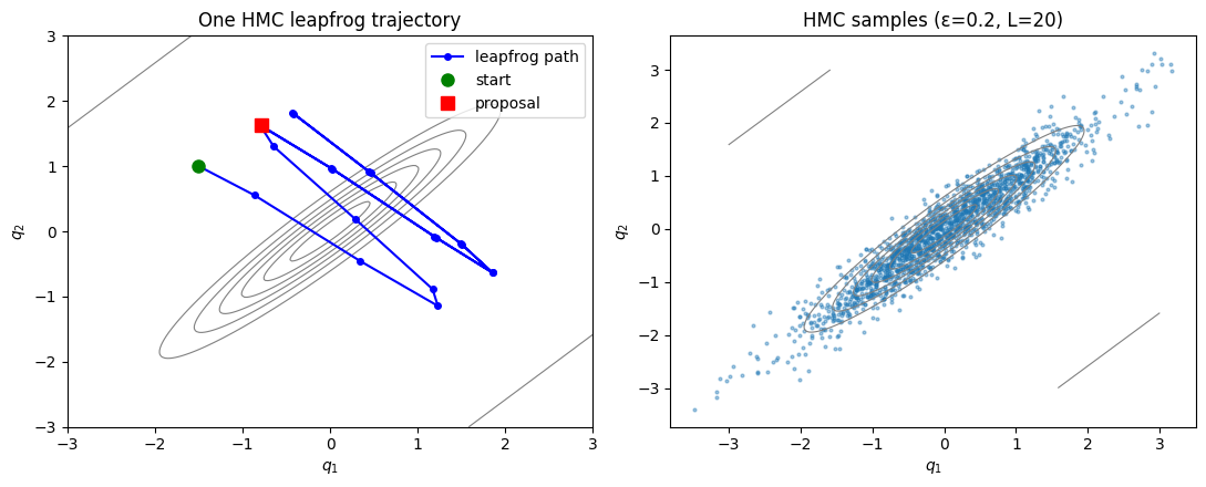

Comparison with Random-Walk MH¶

For random-walk MH on the same target, the proposal s.d. must be small enough to not overshoot the narrow direction ( $\sigma \approx \sqrt{1-\rho^2} \approx 0.31$ ), which makes exploration of the wide direction slow.

# Random-walk MH on same 2D Gaussian
def rwmh(q0, log_joint, σ_prop, num_samples):
    D = q0.shape[0]
    q = q0.clone()
    samples  = [q.clone()]
    n_accept = 0
    for _ in range(num_samples):
        q_prop = q + σ_prop * torch.randn(D)
        log_α  = log_joint(q_prop) - log_joint(q)
        if torch.rand(1).item() < torch.exp(log_α).item():
            q = q_prop
            n_accept += 1
        samples.append(q.clone())
    return torch.stack(samples), n_accept / num_samples

samples_rw, acc_rw = rwmh(q0_2d, log_joint_2d, σ_prop=0.3, num_samples=2000)
print(f'RW-MH acceptance rate: {acc_rw:.2f}')

ess_hmc = effective_sample_size(samples_hmc[None, burnin:, 0]).item()
ess_rw  = effective_sample_size(samples_rw[None,  burnin:, 0]).item()
print(f'ESS q₁ — HMC: {ess_hmc:.0f},  RW-MH: {ess_rw:.0f}  (out of {2000-burnin} samples)')

RW-MH acceptance rate: 0.60
ESS q₁ — HMC: 2939,  RW-MH: 18  (out of 1800 samples)

fig, axs = plt.subplots(2, 2, figsize=(10, 6), sharex='col')

for col, (samps, label) in enumerate([(samples_hmc, 'HMC'), (samples_rw, 'RW-MH')]):
    axs[0, col].plot(samps[burnin:burnin+500, 0].numpy())
    axs[0, col].set_title(f'{label}: trace of $q_1$')
    axs[0, col].set_ylabel(r'$q_1$')
    axs[1, col].plot(samps[burnin:burnin+500, 1].numpy())
    axs[1, col].set_ylabel(r'$q_2$')
    axs[1, col].set_xlabel('Iteration')

plt.tight_layout()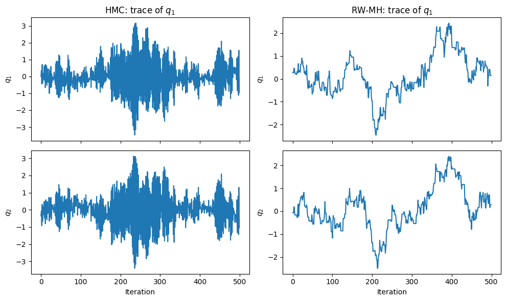

Scaling with Dimension¶

Benefits of Avoiding Random Walks¶

For a $D$ -dimensional isotropic Gaussian target the cost of obtaining one independent sample scales as:

Algorithm	Gradient evaluations
Random-walk MH	$O(D^2)$
MALA	$O(D^{4/3})$
HMC	$O(D^{5/4})$

The advantage of HMC grows with the condition number of the posterior covariance. Random-walk MH must step at the scale of the most constrained dimension, requiring $\kappa$ steps in the widest direction (where $\kappa$ is the condition number). HMC integrates the gradient to traverse the wide direction efficiently in $\sqrt{\kappa}$ leapfrog steps.

Demonstration in Higher Dimensions¶

We compare HMC and random-walk MH on a $D$ -dimensional diagonal Gaussian with eigenvalues linearly spaced from 0.1 to 1 (condition number $= 10$ ).

torch.manual_seed(305)

results = {}
for D in [2, 10, 50, 100]:
    λ_vec = torch.linspace(0.1, 1.0, D)
    Σ_inv_d = torch.diag(1.0 / λ_vec)

    def log_joint_d(q, Σ_inv=Σ_inv_d):
        return -0.5 * q @ Σ_inv @ q

    def grad_U_d(q, Σ_inv=Σ_inv_d):
        return Σ_inv @ q

    # HMC: step size ≈ smallest std, L = 20
    ε_hmc = 0.8 * λ_vec.min().sqrt().item()
    samp_h, _ = hmc(torch.zeros(D), log_joint_d, grad_U_d,
                    ε=ε_hmc, L=20, M=torch.eye(D), num_samples=2000)
    ess_h = effective_sample_size(samp_h[None, 500:, 0]).item()

    # RW-MH: proposal std ≈ smallest std
    samp_r, _ = rwmh(torch.zeros(D), log_joint_d, σ_prop=λ_vec.min().sqrt().item(), num_samples=2000)
    ess_r = effective_sample_size(samp_r[None, 500:, 0]).item()

    results[D] = (ess_h, ess_r)
    print(f'D={D:3d}: ESS HMC={ess_h:6.0f}, ESS RW-MH={ess_r:6.0f}')

D=  2: ESS HMC=  8182, ESS RW-MH=   172

D= 10: ESS HMC=  6103, ESS RW-MH=    92

D= 50: ESS HMC=  5127, ESS RW-MH=    26

D=100: ESS HMC=  3838, ESS RW-MH=   nan

dims = sorted(results)
ess_h_vals = [results[d][0] for d in dims]
ess_r_vals = [results[d][1] for d in dims]

plt.figure(figsize=(6, 4))
plt.plot(dims, ess_h_vals, 's-', label='HMC')
plt.plot(dims, ess_r_vals, 'o-', label='RW-MH')
plt.xlabel('Dimension $D$')
plt.ylabel('ESS (out of 1500 post-burnin samples)')
plt.title('HMC vs. RW-MH effective sample size')
plt.legend()
plt.tight_layout()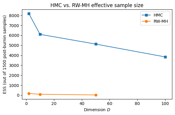

Practical Considerations¶

Step-Size Adaptation¶

The step size $\epsilon$ must be tuned:

Too large → large energy errors → low acceptance rate.
Too small → small moves → slow mixing.

A target acceptance rate of ~0.65 is recommended by Neal, 2011. A simple strategy during warm-up: increase $\epsilon$ when the acceptance rate exceeds the target, decrease when below. The dual averaging scheme of Hoffman & Gelman, 2014 provides a principled adaptive version used by default in Pyro and Stan.

No-U-Turn Sampler¶

Choosing $L$ by hand is also inconvenient. The No-U-Turn Sampler (NUTS) Hoffman & Gelman, 2014 extends the trajectory dynamically until it begins turning back (the inner product $\mbp \cdot (\mbq - {\mbq}_0) < 0$ ), then selects a sample from along the trajectory using slice sampling. NUTS:

Eliminates the need to tune $L$ .
Adapts $\epsilon$ automatically during warm-up.
Is the default backend for Stan, PyMC, and Pyro’s NUTS kernel.

An interactive visualization of HMC and NUTS: https://chi-feng.github.io/mcmc-demo/app.html

Conclusion¶

HMC exploits gradient information to make large, coherent moves through parameter space, vastly outperforming random-walk methods in high dimensions. Key points:

The potential energy is $U(\mbq) = -\log p(\mbq, \mbX)$ ; auxiliary momentum variables $\mbp \sim \cN(\mbzero, \mbM)$ complete the Hamiltonian system.
Hamiltonian dynamics are reversible, energy-conserving, and volume-preserving — exactly the properties needed for a valid MCMC kernel.
The leapfrog integrator preserves these properties approximately, introducing only $O(\epsilon^2)$ energy error per step.
The Metropolis correction accounts for numerical integration error, ensuring exact invariance with respect to the target.
NUTS removes the need to hand-tune $L$ and is the practical choice for most applications.

References¶

Neal, R. M. (2011). MCMC using Hamiltonian dynamics. Handbook of Markov Chain Monte Carlo, 2(11), 2.
Hoffman, M. D., & Gelman, A. (2014). The No-U-Turn sampler: adaptively setting path lengths in Hamiltonian Monte Carlo. Journal of Machine Learning Research, 15(1), 1593–1623.
Betancourt, M. (2017). A conceptual introduction to Hamiltonian Monte Carlo. arXiv Preprint arXiv:1701.02434.