The previous two chapters developed the machinery for gradient-based VI: the ELBO, the reparameterisation trick, and Adam. A Variational Autoencoder (VAE) Kingma & Welling, 2014Rezende et al., 2014 puts these tools to work in a deep generative model. The core idea is simple:
Fit a nonlinear latent variable model by jointly learning a decoder (generative model) and an encoder (approximate posterior) using the reparameterised ELBO.
The result is a model that can both generate new data (by sampling from the prior and decoding) and embed data into a structured latent space (by encoding).
Topics covered:
The VAE generative model: from PPCA to deep latent variable models
The ELBO as reconstruction loss + KL regulariser
Amortised inference: why we use an encoder network instead of per-datapoint variational parameters
The complete training algorithm in a single clean loop
Code: a VAE on 2D data with a 1D latent space
Source
import torch
import torch.nn as nn
import torch.distributions as dist
import matplotlib.pyplot as plt
import matplotlib.cm as cm

palette = list(plt.cm.tab10.colors)
The Generative Model
From PPCA to VAEs
Recall Probabilistic PCA from Chapter 6:
The decoder is linear. A VAE replaces it with a neural network:
where is a multilayer perceptron (MLP) with parameters , and is a suitable observation model (Gaussian for real data, Bernoulli for binary data, etc.).
The prior acts as a regulariser: it encourages the latent space to be compact and well-organised.
Why Is the Posterior Intractable?
In PPCA the posterior is Gaussian and has a closed form. In a VAE, the nonlinear decoder means
is no longer a standard distribution — the normalising constant requires integrating over , which is intractable. This is where variational inference comes in.
The ELBO: Reconstruction + KL
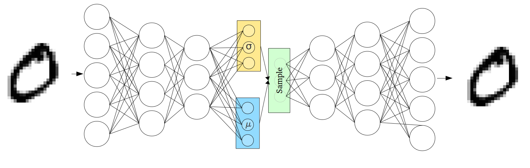
The VAE encoder-decoder architecture. The encoder maps a data point to variational parameters ; the decoder maps a latent sample back to the observation space. The ELBO balances reconstruction quality against the KL regulariser.
Introduce a variational approximation to the intractable posterior. The ELBO for data point is:
This decomposition has a clean interpretation:
| Term | Name | Role |
|---|---|---|
| Reconstruction | How well can we recover from its encoding ? | |
| KL regulariser | How far is the approximate posterior from the prior? |
Maximising the ELBO encourages good reconstructions while keeping the latent codes close to the prior — the same tension as a regularised autoencoder.
Gaussian Encoder and Decoder
Use a diagonal Gaussian encoder . The KL term then has a closed form:
For a Gaussian decoder , the reconstruction term is just
where is the reparameterised noise.
Amortised Inference: The Encoder Network
The Per-Datapoint Bottleneck
With data points we have sets of variational parameters . If we optimise each independently — running many gradient steps on for every update of — the E-step dominates the computation and the method does not scale.
The Key Observation
The optimal variational parameters are a function of the data point:
Instead of learning independent vectors, we learn a single encoder network (also called a recognition network or inference network) that maps any data point to its variational parameters:
Amortisation means we amortise the cost of inference across the entire dataset: one forward pass through the encoder gives instantly, at the cost of a slightly suboptimal approximation.
The Amortisation Gap
The encoder can only represent functions in the parametric class defined by its architecture. This introduces an amortisation gap:
There is also an approximation gap from restricting to the diagonal-Gaussian family. Cremer et al., 2018 study both gaps empirically.
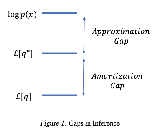
Illustration of the approximation gap (restricting to a parametric family) and the amortisation gap (using a shared encoder instead of per-datapoint optimisation). Figure from Cremer et al., 2018.
The VAE Training Algorithm
With an encoder, the ELBO for data point becomes a function of both (decoder) and (encoder):
Because is reparameterised through via and , the gradient flows through the encoder by standard backpropagation.
The complete algorithm — no separate E and M steps:
repeat:
    sample mini-batch {x_n} ⊂ {x_1, …, x_N}
    for each x_n in the mini-batch:
        compute (μ_φ(x_n), σ_φ(x_n)) via encoder forward pass
        sample ε ~ N(0, I);  z_n = μ_φ(x_n) + σ_φ(x_n) ⊙ ε
        compute ELBO_n = log p(x_n | g(z_n; θ)) − KL term
    loss = −mean(ELBO_n)
    loss.backward()             # gradients wrt both θ and φ
    optimiser.step()            # update θ and φ together
The encoder and decoder are trained jointly in a single optimisation loop — there is no explicit E-step / M-step separation.
# ── Dataset: 2D observations on a noisy 1D manifold (sine curve) ─────────────
torch.manual_seed(305)
N = 1000
t_true = torch.linspace(-3, 3, N) + 0.05 * torch.randn(N) # latent "phase"
X = torch.stack([t_true + 0.15 * torch.randn(N),
torch.sin(t_true) + 0.15 * torch.randn(N)], dim=1) # (N, 2)
# Colour points by their true phase for later visualisation
c_true = t_true.numpy()
# ── Model ─────────────────────────────────────────────────────────────────────
class Encoder(nn.Module):
"""Maps x ∈ R^D to (μ_z, log σ_z) ∈ R^H × R^H."""
def __init__(self, D, H, hidden=32):
super().__init__()
self.net = nn.Sequential(
nn.Linear(D, hidden), nn.Tanh(),
nn.Linear(hidden, hidden), nn.Tanh(),
)
self.mu_head = nn.Linear(hidden, H)
self.logσ_head = nn.Linear(hidden, H)
def forward(self, x):
h = self.net(x)
return self.mu_head(h), self.logσ_head(h)
class Decoder(nn.Module):
"""Maps z ∈ R^H to μ_x ∈ R^D (Gaussian likelihood with unit variance)."""
def __init__(self, H, D, hidden=32):
super().__init__()
self.net = nn.Sequential(
nn.Linear(H, hidden), nn.Tanh(),
nn.Linear(hidden, hidden), nn.Tanh(),
nn.Linear(hidden, D),
)
def forward(self, z):
return self.net(z)
def elbo(x, encoder, decoder):
"""Single-sample reparameterised ELBO (per data point, mean over batch)."""
μ_z, logσ_z = encoder(x) # (B, H)
σ_z = logσ_z.exp()
# Reparameterised sample
ε = torch.randn_like(μ_z)
z = μ_z + σ_z * ε # (B, H)
# Reconstruction: -0.5 ||x - g(z)||^2 (ignoring log 2π constant)
x_hat = decoder(z) # (B, D)
recon = -0.5 * ((x - x_hat) ** 2).sum(dim=1).mean()
# KL[ N(μ_z, diag(σ_z²)) || N(0, I) ] closed form
kl = 0.5 * (μ_z**2 + σ_z**2 - 1 - logσ_z * 2).sum(dim=1).mean()
return recon - kl, recon.item(), kl.item()
# ── Training ──────────────────────────────────────────────────────────────────
H, D = 1, 2 # 1-D latent space, 2-D observations
batch_size = 128
num_epochs = 300
encoder = Encoder(D, H, hidden=32)
decoder = Decoder(H, D, hidden=32)
opt = torch.optim.Adam(list(encoder.parameters()) +
list(decoder.parameters()), lr=1e-3)
dataset = torch.utils.data.TensorDataset(X)
loader = torch.utils.data.DataLoader(dataset, batch_size=batch_size, shuffle=True)
history = {'elbo': [], 'recon': [], 'kl': []}
for epoch in range(num_epochs):
for (xb,) in loader:
lb, r, k = elbo(xb, encoder, decoder)
(-lb).backward()
opt.step(); opt.zero_grad()
# Track once per epoch on full data
with torch.no_grad():
lb_full, r_full, k_full = elbo(X, encoder, decoder)
history['elbo'].append(lb_full)
history['recon'].append(r_full)
history['kl'].append(k_full)
print(f'Final ELBO: {history["elbo"][-1]:.2f} '
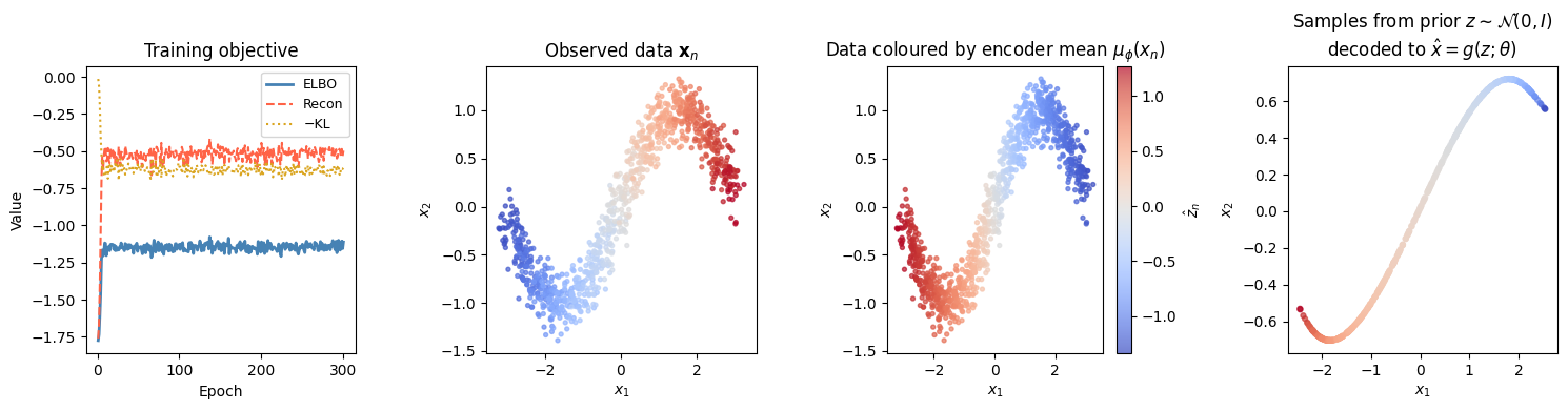
f'(recon={history["recon"][-1]:.2f}, KL={history["kl"][-1]:.2f})')Final ELBO: -1.11 (recon=-0.50, KL=0.61)
Source
fig, axes = plt.subplots(1, 4, figsize=(15, 4))

# ── Panel 1: Training curves ─────────────────────────────────────────────────
ax = axes[0]
ep = range(1, num_epochs + 1)
ax.plot(ep, history['elbo'],  lw=2, color='steelblue', label='ELBO')
ax.plot(ep, history['recon'], lw=1.5, ls='--', color='tomato',   label='Recon')
ax.plot(ep, [-k for k in history['kl']], lw=1.5, ls=':', color='goldenrod', label='−KL')
ax.set_xlabel('Epoch'); ax.set_ylabel('Value')
ax.set_title('Training objective'); ax.legend(fontsize=9)

# ── Panel 2: Original data ────────────────────────────────────────────────────
axes[1].scatter(X[:, 0].numpy(), X[:, 1].numpy(),
                c=c_true, cmap='coolwarm', s=8, alpha=0.7)
axes[1].set_title('Observed data $\mathbf{x}_n$')
axes[1].set_xlabel('$x_1$'); axes[1].set_ylabel('$x_2$')

# ── Panel 3: Latent encoding ──────────────────────────────────────────────────
with torch.no_grad():
    μ_enc, _ = encoder(X)              # (N, H=1)
z_vals = μ_enc[:, 0].numpy()
sc = axes[2].scatter(X[:, 0].numpy(), X[:, 1].numpy(),
                     c=z_vals, cmap='coolwarm', s=8, alpha=0.7)
plt.colorbar(sc, ax=axes[2], label='$\hat{z}_n$')
axes[2].set_title('Data coloured by encoder mean $\mu_\phi(x_n)$')
axes[2].set_xlabel('$x_1$'); axes[2].set_ylabel('$x_2$')

# ── Panel 4: Samples from prior ───────────────────────────────────────────────
with torch.no_grad():
    z_prior = torch.randn(500, H)
    x_gen   = decoder(z_prior)
axes[3].scatter(x_gen[:, 0].numpy(), x_gen[:, 1].numpy(),
                c=z_prior[:, 0].numpy(), cmap='coolwarm', s=12, alpha=0.7)
axes[3].set_title('Samples from prior $z \sim \mathcal{N}(0,I)$\ndecoded to $\hat{x} = g(z;\\theta)$')
axes[3].set_xlabel('$x_1$'); axes[3].set_ylabel('$x_2$')

plt.tight_layout()
<>:15: SyntaxWarning: invalid escape sequence '\m'
<>:24: SyntaxWarning: invalid escape sequence '\h'
<>:25: SyntaxWarning: invalid escape sequence '\m'
<>:34: SyntaxWarning: invalid escape sequence '\s'
<>:15: SyntaxWarning: invalid escape sequence '\m'
<>:24: SyntaxWarning: invalid escape sequence '\h'
<>:25: SyntaxWarning: invalid escape sequence '\m'
<>:34: SyntaxWarning: invalid escape sequence '\s'
/tmp/ipykernel_2733/1691678671.py:15: SyntaxWarning: invalid escape sequence '\m'
axes[1].set_title('Observed data $\mathbf{x}_n$')
/tmp/ipykernel_2733/1691678671.py:24: SyntaxWarning: invalid escape sequence '\h'
plt.colorbar(sc, ax=axes[2], label='$\hat{z}_n$')
/tmp/ipykernel_2733/1691678671.py:25: SyntaxWarning: invalid escape sequence '\m'
axes[2].set_title('Data coloured by encoder mean $\mu_\phi(x_n)$')
/tmp/ipykernel_2733/1691678671.py:34: SyntaxWarning: invalid escape sequence '\s'
axes[3].set_title('Samples from prior $z \sim \mathcal{N}(0,I)$\ndecoded to $\hat{x} = g(z;\\theta)$')
Conclusion
A VAE is a nonlinear latent variable model trained by amortised variational inference.
| Component | Role | Parameters |
|---|---|---|
| Decoder | Generative model: maps latent → observed | |
| Encoder | Recognition model: maps observed → | |
| Prior | Regulariser on the latent space | — |
The ELBO has two interpretable terms:
Key takeaways:
Amortisation replaces separate optimisation problems (one per data point) with a single shared encoder, enabling scalability.
Reparameterisation makes the ELBO differentiable through both the decoder (via ) and the encoder (via ), so both can be trained in a single gradient loop.
The KL term with a standard normal prior has a closed form for diagonal Gaussian encoders, eliminating MC noise from that term.
A linear VAE (linear encoder and decoder) recovers PPCA exactly, so VAEs are a strict generalisation of the linear LVMs from Chapter 6.
Two sources of sub-optimality: the approximation gap (diagonal Gaussian may not match the true posterior shape) and the amortisation gap (the encoder may not perfectly represent the optimal for every ).
- Kingma, D. P., & Welling, M. (2014). Auto-encoding variational Bayes. arXiv Preprint arXiv:1312.6114.
- Rezende, D. J., Mohamed, S., & Wierstra, D. (2014). Stochastic Backpropagation and Approximate Inference in Deep Generative Models.
- Cremer, C., Li, X., & Duvenaud, D. (2018). Inference suboptimality in variational autoencoders. International Conference on Machine Learning, 1078–1086.