Hidden Markov Models

A Hidden Markov Model (HMM) extends the mixture model by allowing the latent state to evolve over time according to a Markov chain. Where a mixture model treats each observation independently, an HMM captures temporal structure: the hidden state at time $t$ depends on the state at time $t-1$ .

This chapter covers:

The HMM generative model
Exact inference via the forward-backward algorithm
Learning parameters with EM (the Baum-Welch algorithm)

<torch._C.Generator at 0x7fe728fdfa30>

From Mixture Models to HMMs¶

Recall the Gaussian mixture model from Chapter 8:

z_t \overset{\mathrm{iid}}{\sim} \mathrm{Cat}(\boldsymbol{\pi}), \qquad \mathbf{x}_t \mid z_t \sim \mathcal{N}(\boldsymbol{\mu}_{z_t}, \boldsymbol{\Sigma}_{z_t}).

(1)

The i.i.d. assumption means each data point is assigned to a cluster independently of its neighbours. For time-series data this is often unrealistic: a speaker stays in the same phoneme for multiple frames; a mouse stays in the same behavioural state for seconds.

The HMM replaces the i.i.d. prior on $z_t$ with a Markov chain:

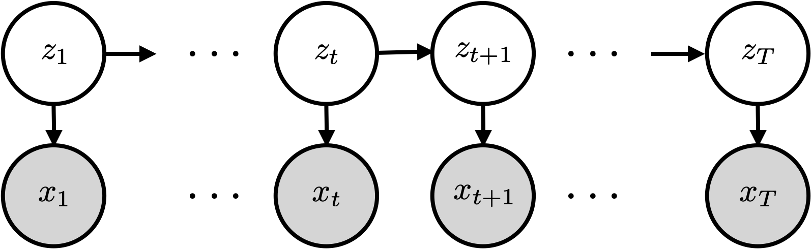
Graphical model for an HMM. The hidden states z_1, z_2, \ldots follow
a Markov chain; each observation \mathbf{x}_t depends only on the
current state z_t. — Graphical model for an HMM. The hidden states $z_1, z_2, \ldots$ follow a Markov chain; each observation $\mathbf{x}_t$ depends only on the current state $z_t$ .

The joint distribution factors as:

p(z_{1:T}, \mathbf{x}_{1:T}) = p(z_1)\prod_{t=2}^T p(z_t \mid z_{t-1})\prod_{t=1}^T p(\mathbf{x}_t \mid z_t).

(2)

We call this an HMM because the hidden states follow a Markov chain, $p(z_1)\prod_{t=2}^T p(z_t \mid z_{t-1})$ .

The Three Components¶

An HMM is defined by three ingredients:

Initial distribution $z_1 \sim \mathrm{Cat}(\boldsymbol{\pi}_0)$ — which state to start in.
Transition matrix $\mathbf{P} \in [0,1]^{K \times K}$ (row-stochastic) — $P_{ij} = p(z_{t+1}=j \mid z_t=i)$ .
Emission distribution $\mathbf{x}_t \sim p(\cdot \mid \boldsymbol{\theta}_{z_t})$ — Gaussian, categorical, Poisson, etc.

Example: The Dishonest Casino¶

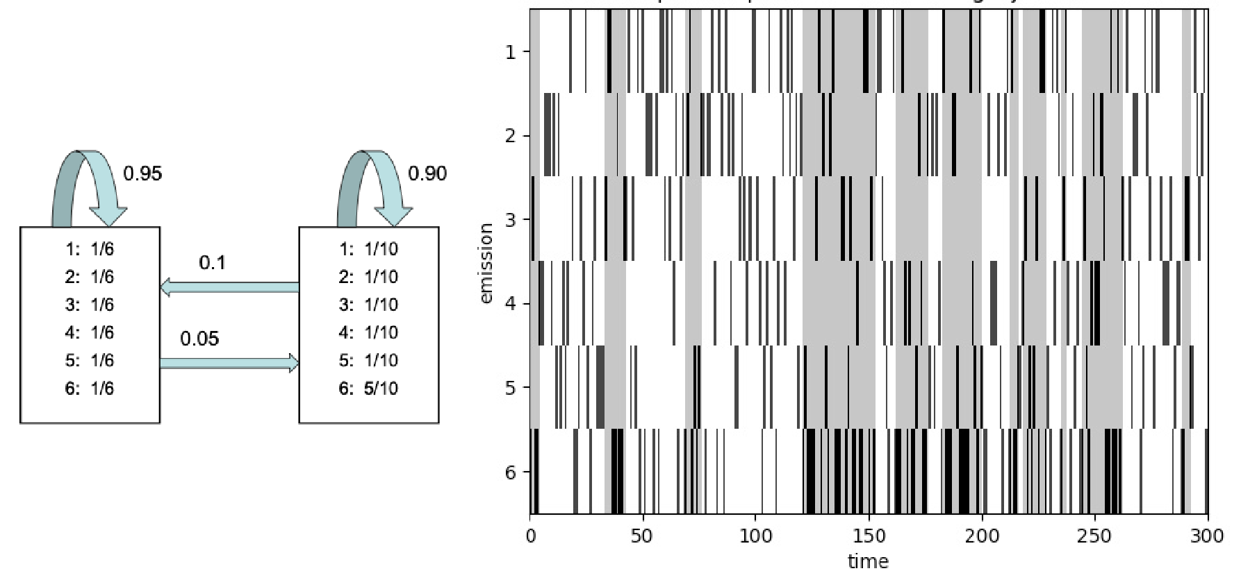
An occasionally dishonest casino that switches between a fair die
(p_k = 1/6) and a loaded die (p_6 = 1/2, p_{1:5} = 1/10).
Figure from dynamax. — An *occasionally* dishonest casino that switches between a fair die ( $p_k = 1/6$ ) and a loaded die ( $p_6 = 1/2$ , $p_{1:5} = 1/10$ ). Figure from dynamax.

Example: Splice Site Recognition¶

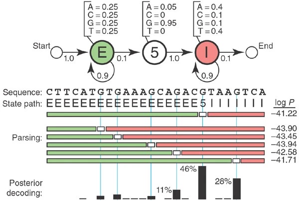
A toy HMM for parsing a genome to find 5'' splice sites.
Figure from . — A toy HMM for parsing a genome to find 5'' splice sites. Figure from Eddy, 2004.

Example: Behavioural Segmentation of Video¶

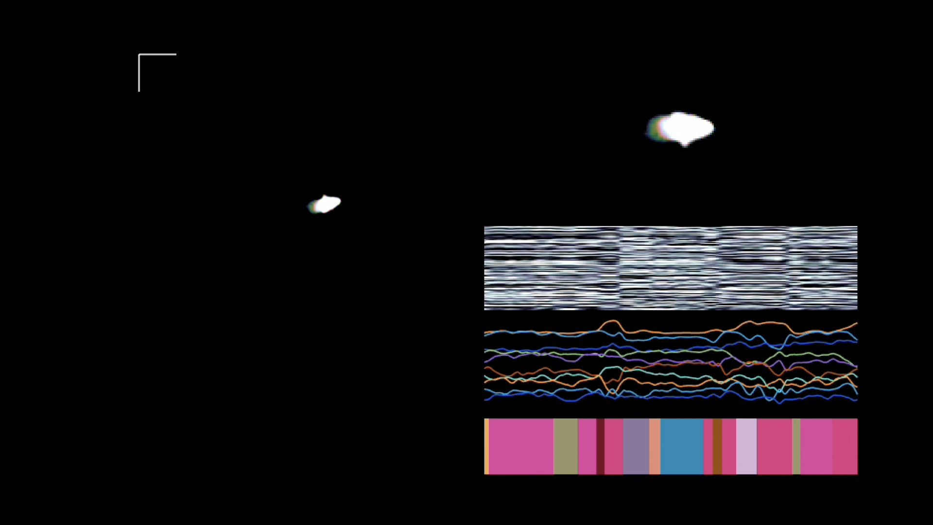
Segmenting videos of freely moving mice with an autoregressive HMM.
Figure from . — Segmenting videos of freely moving mice with an autoregressive HMM. Figure from Wiltschko *et al.*, 2015.

Inference Goals¶

Given observations $\mathbf{x}_{1:T}$ and parameters $\boldsymbol{\Theta}$ , we want:

Quantity	Name
$p(z_t \mid \mathbf{x}_{1:t})$	Filtering — current state given past
$p(z_t \mid \mathbf{x}_{1:T})$	Smoothing — current state given all data
$p(z_t, z_{t+1} \mid \mathbf{x}_{1:T})$	Pairwise smoothing — needed for EM
$\arg\max_{z_{1:T}} p(z_{1:T} \mid \mathbf{x}_{1:T})$	Viterbi — most likely path
$p(\mathbf{x}_{1:T})$	Marginal likelihood — needed for learning

Why is naive enumeration expensive? Marginalising $z_{1:T}$ requires summing over $K^T$ state sequences. Message passing reduces this to $O(TK^2)$ by processing one time step at a time, exploiting the Markov structure.

The Forward Algorithm¶

Define the forward message at time $t$ as the joint probability of being in state $z_t$ and observing $\mathbf{x}_{1:t-1}$ :

\alpha_t(z_t) \triangleq p(z_t,\, \mathbf{x}_{1:t-1}).

(3)

Base case: $\alpha_1(z_1) = p(z_1) = \pi_{0,z_1}$ .

Recursion:

\alpha_{t+1}(z_{t+1}) = \sum_{z_t=1}^K \alpha_t(z_t)\, p(\mathbf{x}_t \mid z_t)\, p(z_{t+1} \mid z_t).

(4)

Let $\boldsymbol{\ell}_t = [p(\mathbf{x}_t \mid z_t=1),\ldots,p(\mathbf{x}_t \mid z_t=K)]^\top$ . In matrix form:

\boldsymbol{\alpha}_{t+1} = \mathbf{P}^\top (\boldsymbol{\alpha}_t \odot \boldsymbol{\ell}_t).

(5)

Normalizing for numerical stability. Re-normalize after each step:

\tilde{\boldsymbol{\alpha}}_{t+1} = \frac{\mathbf{P}^\top(\tilde{\boldsymbol{\alpha}}_t \odot \boldsymbol{\ell}_t)}{A_t}, \qquad A_t = \sum_k \tilde{\alpha}_{t,k}\,\ell_{t,k}.

(6)

The normalizers have a clean interpretation: $\tilde{\boldsymbol{\alpha}}_{t+1}$ is the predictive distribution $p(z_{t+1} \mid \mathbf{x}_{1:t})$ , and $A_t = p(\mathbf{x}_t \mid \mathbf{x}_{1:t-1})$ . Therefore:

\log p(\mathbf{x}_{1:T}) = \sum_{t=1}^T \log A_t.

(7)

The Backward Algorithm and Smoothing¶

Define the backward message as the probability of future observations given the current state:

\beta_t(z_t) \triangleq \sum_{z_{t+1},\ldots,z_T} \prod_{u=t+1}^T p(z_u \mid z_{u-1})\, p(\mathbf{x}_u \mid z_u).

(8)

Base case: $\beta_T(z_T) = 1$ for all $z_T$ .

Recursion:

\beta_t(z_t) = \sum_{z_{t+1}=1}^K p(z_{t+1} \mid z_t)\, p(\mathbf{x}_{t+1} \mid z_{t+1})\, \beta_{t+1}(z_{t+1}),

(9)

or in matrix form: $\boldsymbol{\beta}_t = \mathbf{P}(\boldsymbol{\beta}_{t+1} \odot \boldsymbol{\ell}_{t+1})$ .

Posterior Marginals (Smoothing)¶

p(z_t = k \mid \mathbf{x}_{1:T}) \;\propto\; \alpha_t(k)\, \ell_{t,k}\, \beta_t(k).

(10)

Together the forward and backward passes give the forward-backward algorithm Rabiner & Juang, 1986.

Posterior Pairwise Marginals¶

p(z_t=i,\, z_{t+1}=j \mid \mathbf{x}_{1:T}) \;\propto\; \alpha_t(i)\, \ell_{t,i}\, P_{ij}\, \ell_{t+1,j}\, \beta_{t+1}(j).

(11)

These are needed for the EM M-step below.

EM for HMMs (Baum-Welch)¶

The ELBO for an HMM decomposes over the three parameter groups:

\mathcal{L}(\boldsymbol{\Theta}) = \underbrace{\sum_{k} \gamma_1(k) \log \pi_{0,k}}_{\text{initial dist.}} + \underbrace{\sum_{t=1}^{T-1}\sum_{i,j} \xi_t(i,j) \log P_{ij}}_{\text{transitions}} + \underbrace{\sum_{t=1}^T\sum_{k} \gamma_t(k) \log p(\mathbf{x}_t; \boldsymbol{\theta}_k)}_{\text{emissions}}

(12)

where $\gamma_t(k) = p(z_t=k \mid \mathbf{x}_{1:T})$ (posterior marginals) and $\xi_t(i,j) = p(z_t=i, z_{t+1}=j \mid \mathbf{x}_{1:T})$ (posterior pairwise marginals).

E-step: Run the forward-backward algorithm to compute $\gamma_t$ and $\xi_t$ .

M-step: The ELBO separates, giving closed-form updates:

\hat{\pi}_{0,k} \propto \gamma_1(k), \qquad \hat{P}_{ij} \propto \sum_{t=1}^{T-1} \xi_t(i,j), \qquad \hat{\boldsymbol{\theta}}_k = \text{weighted MLE with weights } \{\gamma_t(k)\}.

(13)

For exponential family emissions, the weighted MLE for $\hat{\boldsymbol{\theta}}_k$ requires only the expected sufficient statistics — the same structure as the mixture model M-step.

# ── Forward-backward algorithm ────────────────────────────────────────────────

def forward_pass(log_pi0, log_P, log_likes):
    '''Normalized forward messages.

    Convention (matching the lecture):
        log_alphas[t, k]  =  log p(z_t=k | x_{0:t-1})   (predictive, normalized)
        log_norms[t]      =  log p(x_t | x_{0:t-1})

    Args:
        log_pi0:   (K,)   log initial distribution
        log_P:     (K, K) log_P[i,j] = log p(z_{t+1}=j | z_t=i)
        log_likes: (T, K) log p(x_t | z_t=k)
    Returns:
        log_alphas (T, K), log_norms (T,)
    '''
    T, K = log_likes.shape
    log_alphas = torch.zeros(T, K)
    log_norms  = torch.zeros(T)

    log_alphas[0] = log_pi0 - torch.logsumexp(log_pi0, 0)
    log_norms[0]  = torch.logsumexp(log_alphas[0] + log_likes[0], 0)

    for t in range(1, T):
        log_joint   = log_alphas[t-1] + log_likes[t-1]              # (K,)
        log_alpha_t = torch.logsumexp(log_joint[:, None] + log_P, 0) # (K,)
        log_alphas[t] = log_alpha_t - torch.logsumexp(log_alpha_t, 0)
        log_norms[t]  = torch.logsumexp(log_alphas[t] + log_likes[t], 0)

    return log_alphas, log_norms


def backward_pass(log_P, log_likes):
    '''Normalized backward messages.

    Args:
        log_P:     (K, K)
        log_likes: (T, K)
    Returns:
        log_betas (T, K),  with log_betas[T-1] = 0 (base case beta_T = 1)
    '''
    T, K = log_likes.shape
    log_betas = torch.zeros(T, K)   # base: beta_{T-1} = 1

    for t in range(T - 2, -1, -1):
        log_joint   = log_likes[t+1] + log_betas[t+1]               # (K,)
        log_beta_t  = torch.logsumexp(log_P + log_joint[None, :], 1) # (K,)
        log_betas[t] = log_beta_t - torch.logsumexp(log_beta_t, 0)

    return log_betas


def posterior_marginals(log_alphas, log_betas, log_likes):
    '''gamma_t(k) = p(z_t=k | x_{0:T-1}).  Returns (T, K).'''
    log_gamma = log_alphas + log_likes + log_betas
    log_gamma = log_gamma - torch.logsumexp(log_gamma, 1, keepdim=True)
    return log_gamma.exp()


def posterior_pairs(log_alphas, log_betas, log_likes, log_P):
    '''xi_t(i,j) = p(z_t=i, z_{t+1}=j | x_{0:T-1}).  Returns (T-1, K, K).'''
    T, K = log_alphas.shape
    log_xi = (log_alphas[:-1, :, None]
              + log_likes[:-1, :, None]
              + log_P[None]
              + log_likes[1:, None, :]
              + log_betas[1:, None, :])
    log_xi = log_xi - torch.logsumexp(log_xi.reshape(T-1, -1), 1).reshape(T-1, 1, 1)
    return log_xi.exp()


# ── EM for an HMM with categorical emissions ──────────────────────────────────

def cat_log_likes(x, log_theta):
    '''log p(x_t | z_t=k) for categorical emissions.

    Args:
        x:         (T,)    integer observations in {0, ..., V-1}
        log_theta: (K, V)  log emission probabilities
    Returns:
        (T, K)
    '''
    return log_theta[:, x].T


def em_hmm_cat(x, K, V, num_iters=60, seed=0):
    '''Baum-Welch EM for a categorical-emission HMM.

    Args:
        x:         (T,)  integer observations in {0, ..., V-1}
        K:         number of hidden states
        V:         vocabulary size (number of emission symbols)
        num_iters: EM iterations
    Returns:
        pi0 (K,), P (K, K), theta (K, V), ll_history
    '''
    torch.manual_seed(seed)
    T = len(x)

    # Random initialisation
    pi0   = torch.ones(K) / K
    P     = torch.ones(K, K) / K
    theta = torch.rand(K, V)
    theta = theta / theta.sum(1, keepdim=True)

    ll_history = []

    for _ in range(num_iters):
        # E-step
        log_ll        = cat_log_likes(x, theta.log())
        log_alphas, log_norms = forward_pass(pi0.log(), P.log(), log_ll)
        log_betas     = backward_pass(P.log(), log_ll)
        gamma         = posterior_marginals(log_alphas, log_betas, log_ll)  # (T, K)
        xi            = posterior_pairs(log_alphas, log_betas, log_ll, P.log())  # (T-1,K,K)

        ll_history.append(log_norms.sum().item())

        # M-step
        pi0   = (gamma[0] + 1e-8) / (gamma[0] + 1e-8).sum()

        xi_sum = xi.sum(0) + 1e-8                                    # (K, K)
        P      = xi_sum / xi_sum.sum(1, keepdim=True)

        # Weighted counts for each emission symbol
        x_oh  = torch.zeros(T, V).scatter_(1, x.unsqueeze(1), 1.0)  # (T, V) one-hot
        counts = gamma.T @ x_oh + 1e-8                               # (K, V)
        theta  = counts / counts.sum(1, keepdim=True)

    return pi0, P, theta, ll_history

# ── Simulate from the dishonest casino ───────────────────────────────────────
K_true = 2     # states: 0=fair, 1=loaded
V      = 6     # die faces 0..5
T_sim  = 300

pi0_true   = torch.tensor([1.0, 0.0])
P_true     = torch.tensor([[0.95, 0.05],
                            [0.10, 0.90]])
theta_true = torch.tensor([[1/6]*6,
                           [0.1, 0.1, 0.1, 0.1, 0.1, 0.5]])

torch.manual_seed(42)
z_true = torch.zeros(T_sim, dtype=torch.long)
x_obs  = torch.zeros(T_sim, dtype=torch.long)
z_true[0] = dist.Categorical(pi0_true).sample()
x_obs[0]  = dist.Categorical(theta_true[z_true[0]]).sample()
for t in range(1, T_sim):
    z_true[t] = dist.Categorical(P_true[z_true[t-1]]).sample()
    x_obs[t]  = dist.Categorical(theta_true[z_true[t]]).sample()

# ── Run EM to learn parameters ───────────────────────────────────────────────
pi0_em, P_em, theta_em, ll_hist = em_hmm_cat(x_obs, K=2, V=6, num_iters=80)

# Align states (EM may swap labels)
# State with higher p(6) should be "loaded"
loaded = theta_em[:, 5].argmax().item()
fair   = 1 - loaded

# Posterior marginals with learned parameters
log_ll_em    = cat_log_likes(x_obs, theta_em.log())
la, ln       = forward_pass(pi0_em.log(), P_em.log(), log_ll_em)
lb           = backward_pass(P_em.log(), log_ll_em)
gamma_em     = posterior_marginals(la, lb, log_ll_em)

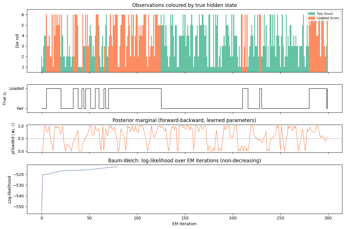
# ── Plot ──────────────────────────────────────────────────────────────────────
fig, axes = plt.subplots(4, 1, figsize=(12, 8), sharex=True,
                         gridspec_kw={'height_ratios': [1.8, 0.8, 0.8, 1.4]})

# Panel 1: die rolls coloured by true state
ax = axes[0]
colors = [palette[0] if z_true[t] == 0 else palette[1] for t in range(T_sim)]
ax.bar(range(T_sim), x_obs.numpy() + 1, color=colors, width=1.0, linewidth=0)
ax.set_ylabel('Die roll')
ax.set_ylim(0.5, 6.5)
ax.set_yticks([1, 2, 3, 4, 5, 6])
ax.set_title('Observations coloured by true hidden state')
fair_patch   = mpatches.Patch(color=palette[0], label='Fair (true)')
loaded_patch = mpatches.Patch(color=palette[1], label='Loaded (true)')
ax.legend(handles=[fair_patch, loaded_patch], loc='upper right', fontsize=8)

# Panel 2: true hidden state sequence
ax = axes[1]
ax.step(range(T_sim), z_true.numpy(), where='post', color='k', lw=0.9)
ax.set_ylabel('True $z_t$')
ax.set_ylim(-0.2, 1.2)
ax.set_yticks([0, 1])
ax.set_yticklabels(['Fair', 'Loaded'])

# Panel 3: posterior p(loaded | all data) using learned parameters
ax = axes[2]
ax.plot(range(T_sim), gamma_em[:, loaded].numpy(), color=palette[1], lw=1.1)
ax.axhline(0.5, color='gray', linestyle='--', lw=0.7)
ax.set_ylabel('$p(\mathrm{loaded} \mid \mathbf{x}_{1:T})$')
ax.set_ylim(-0.05, 1.05)
ax.set_title('Posterior marginal (forward-backward, learned parameters)')

# Panel 4: ELBO / log-likelihood over EM iterations
ax = axes[3]
ax.plot(ll_hist, color=palette[2], lw=1.5)
ax.set_xlabel('EM iteration')
ax.set_ylabel('Log-likelihood')
ax.set_title('Baum-Welch: log-likelihood over EM iterations (non-decreasing)')

plt.tight_layout()
plt.show()

# Print learned vs true emission probabilities
print("Learned emission probs (fair die)  :", theta_em[fair].numpy().round(3))
print("True emission probs   (fair die)  :", theta_true[0].numpy().round(3))
print()
print("Learned emission probs (loaded die):", theta_em[loaded].numpy().round(3))
print("True emission probs   (loaded die):", theta_true[1].numpy().round(3))
print()
print(f"Learned transition matrix:\n{P_em.numpy().round(3)}")
print(f"True transition matrix:\n{P_true.numpy()}")

<>:63: SyntaxWarning: invalid escape sequence '\m'
<>:63: SyntaxWarning: invalid escape sequence '\m'

/tmp/ipykernel_2718/3219947313.py:63: SyntaxWarning: invalid escape sequence '\m'
  ax.set_ylabel('$p(\mathrm{loaded} \mid \mathbf{x}_{1:T})$')

Learned emission probs (fair die)  : [0.304 0.209 0.193 0.    0.02  0.274]
True emission probs   (fair die)  : [0.167 0.167 0.167 0.167 0.167 0.167]

Learned emission probs (loaded die): [0.002 0.101 0.149 0.236 0.201 0.311]
True emission probs   (loaded die): [0.1 0.1 0.1 0.1 0.1 0.5]

Learned transition matrix:
[[0.703 0.297]
 [0.188 0.812]]
True transition matrix:
[[0.95 0.05]
 [0.1  0.9 ]]

Conclusion¶

Component	Key idea
HMM	Mixture model with a Markov prior on $z_t$
Forward pass	Recursive $O(TK^2)$ computation of $p(z_t, \mathbf{x}_{1:t-1})$
Backward pass	Recursive $O(TK^2)$ computation of $p(\mathbf{x}_{t+1:T} \mid z_t)$
Forward-backward	Combines both to give $p(z_t \mid \mathbf{x}_{1:T})$
Baum-Welch / EM	E-step = forward-backward; M-step = weighted MLE

Extensions worth knowing:

Viterbi algorithm: replaces $\sum$ with $\max$ to find the most likely state sequence $\arg\max_{z_{1:T}} p(z_{1:T} \mid \mathbf{x}_{1:T})$ .
Autoregressive HMMs: each emission depends on both $z_t$ and recent observations $\mathbf{x}_{t-1}$ Wiltschko et al., 2015.
Bayesian HMMs: place a Dirichlet prior on $\boldsymbol{\pi}_0$ , rows of $\mathbf{P}$ , and emission parameters; use Gibbs sampling or VI.
Infinite HMMs (iHMMs): nonparametric prior lets the number of states grow with the data.