Linear Dynamical Systems

The previous chapter introduced Hidden Markov Models, where the hidden state $z_t$ was discrete. Here we keep the same graphical model but allow $\mathbf{z}_t \in \mathbb{R}^{D_z}$ to be continuous. When both the dynamics and the emissions are Gaussian and linear, the model is called a Linear Dynamical System (LDS), also known as a linear Gaussian state space model. The key payoff is that the forward-backward algorithm reduces to a pair of closed-form matrix recursions: the Kalman filter Kalman, 1960 and the Rauch-Tung-Striebel (RTS) smoother Rauch et al., 1965.

import torch
import torch.distributions as dist
import matplotlib.pyplot as plt
import matplotlib.patches as mpatches
from matplotlib.patches import Ellipse
import numpy as np

palette = list(plt.cm.Set2.colors)
torch.manual_seed(305)

<torch._C.Generator at 0x7f7ff41bf9f0>

From HMMs to State Space Models¶

An HMM uses the same graphical model as a general state space model:

p(\mathbf{z}_{1:T}, \mathbf{x}_{1:T}) = p(\mathbf{z}_1)\prod_{t=2}^T p(\mathbf{z}_t \mid \mathbf{z}_{t-1}) \prod_{t=1}^T p(\mathbf{x}_t \mid \mathbf{z}_t).

(1)

In an HMM, $z_t \in \{1,\ldots,K\}$ is discrete and the forward-backward algorithm sweeps over $K$ values at each time step. Nothing in the graphical model requires discrete states, however. If $\mathbf{z}_t$ is continuous, the sums in the forward-backward recursions become integrals. In general those integrals are intractable, but for the Gaussian linear case they have a closed form.

The Linear Dynamical System¶

The LDS is defined by Gaussian dynamics and Gaussian emissions:

\mathbf{z}_1 \sim \mathcal{N}(\boldsymbol{\mu}_0, \boldsymbol{\Sigma}_0)

(2)

\mathbf{z}_t \mid \mathbf{z}_{t-1} \sim \mathcal{N}(\mathbf{A}\mathbf{z}_{t-1} + \mathbf{b},\; \mathbf{Q}) \qquad t = 2,\ldots,T

(3)

\mathbf{x}_t \mid \mathbf{z}_t \sim \mathcal{N}(\mathbf{C}\mathbf{z}_t + \mathbf{d},\; \mathbf{R}) \qquad t = 1,\ldots,T

(4)

Symbol	Dimension	Role
$\mathbf{A}$	$D_z \times D_z$	Dynamics (transition) matrix
$\mathbf{b}$	$D_z$	Dynamics bias
$\mathbf{Q}$	$D_z \times D_z$	Dynamics noise covariance
$\mathbf{C}$	$D_x \times D_z$	Emission (observation) matrix
$\mathbf{d}$	$D_x$	Emission bias
$\mathbf{R}$	$D_x \times D_x$	Emission noise covariance

Special cases. Setting $\mathbf{A} = \mathbf{0}$ and $\mathbf{Q} = \mathbf{I}$ recovers Probabilistic PCA (Chapter 6): the latent states are i.i.d. Gaussians. The LDS adds temporal dependence through the dynamics matrix $\mathbf{A}$ .

Stability. The dynamics are stable iff all eigenvalues of $\mathbf{A}$ satisfy $|\lambda_i| < 1$ . If any eigenvalue exceeds 1 in magnitude, the latent state diverges.

The Kalman Filter¶

The forward pass for the LDS is the Kalman filter, which computes the filtering distributions

p(\mathbf{z}_t \mid \mathbf{x}_{1:t}) = \mathcal{N}(\mathbf{z}_t \mid \boldsymbol{\mu}_{t|t},\, \boldsymbol{\Sigma}_{t|t})

(5)

via two alternating steps. Assuming the predicted distribution $p(\mathbf{z}_t \mid \mathbf{x}_{1:t-1}) = \mathcal{N}(\boldsymbol{\mu}_{t|t-1}, \boldsymbol{\Sigma}_{t|t-1})$ is in hand, we proceed as follows.

Update Step¶

Condition on the new observation $\mathbf{x}_t$ . The joint distribution of $(\mathbf{z}_t, \mathbf{x}_t)$ given $\mathbf{x}_{1:t-1}$ is jointly Gaussian:

\begin{pmatrix}\mathbf{z}_t \\ \mathbf{x}_t\end{pmatrix} \Bigg|\, \mathbf{x}_{1:t-1} \sim \mathcal{N}\!\left( \begin{pmatrix}\boldsymbol{\mu}_{t|t-1} \\ \mathbf{C}\boldsymbol{\mu}_{t|t-1}+\mathbf{d}\end{pmatrix},\; \begin{pmatrix} \boldsymbol{\Sigma}_{t|t-1} & \boldsymbol{\Sigma}_{t|t-1}\mathbf{C}^\top \\ \mathbf{C}\boldsymbol{\Sigma}_{t|t-1} & \mathbf{C}\boldsymbol{\Sigma}_{t|t-1}\mathbf{C}^\top + \mathbf{R} \end{pmatrix} \right).

(6)

Applying the conditional Gaussian formula (Chapter 2), the posterior is:

\boldsymbol{\mu}_{t|t} = \boldsymbol{\mu}_{t|t-1} + \mathbf{K}_t\,\boldsymbol{\delta}_t, \qquad \boldsymbol{\Sigma}_{t|t} = (\mathbf{I} - \mathbf{K}_t\mathbf{C})\,\boldsymbol{\Sigma}_{t|t-1}

(7)

where

\boldsymbol{\delta}_t = \mathbf{x}_t - \mathbf{C}\boldsymbol{\mu}_{t|t-1} - \mathbf{d} \qquad\text{(innovation)}

(8)

\mathbf{S}_t = \mathbf{C}\boldsymbol{\Sigma}_{t|t-1}\mathbf{C}^\top + \mathbf{R} \qquad\text{(innovation covariance)}

(9)

\mathbf{K}_t = \boldsymbol{\Sigma}_{t|t-1}\mathbf{C}^\top\mathbf{S}_t^{-1} \qquad\text{(Kalman gain)}

(10)

The Kalman gain $\mathbf{K}_t$ interpolates between the prior prediction and the observation: when $\mathbf{R} \to 0$ (perfect sensors) $\mathbf{K}_t \to \mathbf{C}^{-1}$ and we trust the data entirely; when $\mathbf{R} \to \infty$ (useless sensors) $\mathbf{K}_t \to 0$ and we ignore the data.

Predict Step¶

Marginalise over $\mathbf{z}_t$ to obtain the predicted distribution for time $t+1$ :

\boldsymbol{\mu}_{t+1|t} = \mathbf{A}\boldsymbol{\mu}_{t|t} + \mathbf{b}, \qquad \boldsymbol{\Sigma}_{t+1|t} = \mathbf{A}\boldsymbol{\Sigma}_{t|t}\mathbf{A}^\top + \mathbf{Q}.

(11)

Base case: $\boldsymbol{\mu}_{1|0} = \boldsymbol{\mu}_0$ and $\boldsymbol{\Sigma}_{1|0} = \boldsymbol{\Sigma}_0$ .

Marginal Likelihood¶

As a byproduct, each update step gives the one-step predictive likelihood:

p(\mathbf{x}_t \mid \mathbf{x}_{1:t-1}) = \mathcal{N}(\mathbf{x}_t \mid \mathbf{C}\boldsymbol{\mu}_{t|t-1}+\mathbf{d},\; \mathbf{S}_t),

(12)

so $\log p(\mathbf{x}_{1:T}) = \sum_{t=1}^T \log p(\mathbf{x}_t \mid \mathbf{x}_{1:t-1})$ .

The RTS Smoother¶

The Kalman filter only uses past observations; it produces the filtering distribution $p(\mathbf{z}_t \mid \mathbf{x}_{1:t})$ . The smoothing distribution $p(\mathbf{z}_t \mid \mathbf{x}_{1:T})$ uses all observations and is generally tighter.

Backward Recursion¶

By the Markov property, $\mathbf{z}_t$ is conditionally independent of $\mathbf{x}_{t+1:T}$ given $\mathbf{z}_{t+1}$ . This gives:

p(\mathbf{z}_t \mid \mathbf{z}_{t+1}, \mathbf{x}_{1:T}) = p(\mathbf{z}_t \mid \mathbf{z}_{t+1}, \mathbf{x}_{1:t}) = \frac{p(\mathbf{z}_t \mid \mathbf{x}_{1:t})\, p(\mathbf{z}_{t+1} \mid \mathbf{z}_t)}{p(\mathbf{z}_{t+1} \mid \mathbf{x}_{1:t})}.

(13)

Marginalising over $\mathbf{z}_{t+1}$ :

p(\mathbf{z}_t \mid \mathbf{x}_{1:T}) = p(\mathbf{z}_t \mid \mathbf{x}_{1:t}) \int \frac{p(\mathbf{z}_{t+1} \mid \mathbf{z}_t)\, p(\mathbf{z}_{t+1} \mid \mathbf{x}_{1:T})}{p(\mathbf{z}_{t+1} \mid \mathbf{x}_{1:t})} \, d\mathbf{z}_{t+1}.

(14)

For the Gaussian LDS all three factors are Gaussian and the integral is tractable. The result is the Rauch-Tung-Striebel (RTS) smoother:

p(\mathbf{z}_t \mid \mathbf{x}_{1:T}) = \mathcal{N}(\boldsymbol{\mu}_{t|T},\, \boldsymbol{\Sigma}_{t|T})

(15)

with backward recursion (starting from $\boldsymbol{\mu}_{T|T}$ , $\boldsymbol{\Sigma}_{T|T}$ from the filter):

\mathbf{G}_t = \boldsymbol{\Sigma}_{t|t}\mathbf{A}^\top \boldsymbol{\Sigma}_{t+1|t}^{-1}

(16)

\boldsymbol{\mu}_{t|T} = \boldsymbol{\mu}_{t|t} + \mathbf{G}_t(\boldsymbol{\mu}_{t+1|T} - \boldsymbol{\mu}_{t+1|t})

(17)

\boldsymbol{\Sigma}_{t|T} = \boldsymbol{\Sigma}_{t|t} + \mathbf{G}_t(\boldsymbol{\Sigma}_{t+1|T} - \boldsymbol{\Sigma}_{t+1|t})\mathbf{G}_t^\top

(18)

The smoother gain $\mathbf{G}_t$ plays the same role as the Kalman gain: it determines how much the smoothed estimate at time $t$ is adjusted based on new information from time $t+1$ .

Information Form and Sparse Linear Algebra¶

There is an elegant alternative view. Write the joint posterior as:

p(\mathbf{z}_{1:T} \mid \mathbf{x}_{1:T}) \propto \mathcal{N}(\mathbf{z}_1 \mid \boldsymbol{\mu}_0, \boldsymbol{\Sigma}_0) \prod_{t=2}^T \mathcal{N}(\mathbf{z}_t \mid \mathbf{A}\mathbf{z}_{t-1}+\mathbf{b}, \mathbf{Q}) \prod_{t=1}^T \mathcal{N}(\mathbf{x}_t \mid \mathbf{C}\mathbf{z}_t+\mathbf{d}, \mathbf{R}).

(19)

Expanding and collecting, the exponent is a quadratic form in $\mathbf{z}_{1:T} \in \mathbb{R}^{T D_z}$ , so the posterior is a multivariate Gaussian with natural parameters $\mathbf{J} \in \mathbb{R}^{TD_z \times TD_z}$ (precision matrix) and $\mathbf{h} \in \mathbb{R}^{TD_z}$ .

The key structural observation is that $\mathbf{J}$ is block-tridiagonal: only the diagonal blocks $\mathbf{J}_{t,t}$ and the off-diagonal blocks $\mathbf{J}_{t,t+1}$ are non-zero, reflecting the Markov structure. The posterior mean $\mathbf{J}^{-1}\mathbf{h}$ can therefore be computed in $O(T D_z^3)$ rather than the naive $O(T^3 D_z^3)$ by exploiting the block-tridiagonal sparsity — and this block-tridiagonal solve is exactly equivalent to the Kalman filter and RTS smoother.

Beyond the Linear Gaussian Case¶

For nonlinear dynamics $\mathbf{z}_t = f(\mathbf{z}_{t-1}) + \text{noise}$ or non-Gaussian noise, the Kalman filter no longer applies exactly. Common approximations include:

Method	Idea
Extended Kalman Filter (EKF)	Linearise $f$ around the current estimate
Unscented Kalman Filter (UKF)	Propagate a set of sigma points through $f$
Sequential Monte Carlo (SMC)	Represent $p(\mathbf{z}_t \mid \mathbf{x}_{1:t})$ by weighted particles

Sequential Monte Carlo. The forward messages are proportional to the predictive distributions $p(\mathbf{z}_t \mid \mathbf{x}_{1:t-1})$ . We can approximate this distribution with $S$ weighted particles $\{(\mathbf{z}_t^{(s)}, w_t^{(s)})\}$ :

Sample $\mathbf{z}_t^{(s)} \sim p(\mathbf{z}_t \mid \mathbf{z}_{t-1}^{(s)})$ (propagate particles).
Weight $w_t^{(s)} = p(\mathbf{x}_t \mid \mathbf{z}_t^{(s)})$ (score against observation).
Normalise and resample with replacement according to $\bar{w}_t^{(s)}$ .

The marginal likelihood is approximated by $\log p(\mathbf{x}_{1:T}) \approx \sum_t \log \frac{1}{S}\sum_s w_t^{(s)}$ .

# ── Kalman filter ─────────────────────────────────────────────────────────────

def kalman_filter(y, A, b, Q, C, d, R, mu0, Sigma0):
    '''Kalman filter for a linear Gaussian SSM.

    Model:
        z_1      ~ N(mu0, Sigma0)
        z_t|z_{t-1} ~ N(A z_{t-1} + b, Q)
        x_t|z_t  ~ N(C z_t + d, R)

    Args:
        y:      (T, Dx)  observations
        A:      (Dz, Dz) dynamics matrix
        b:      (Dz,)    dynamics bias
        Q:      (Dz, Dz) dynamics noise covariance
        C:      (Dx, Dz) emission matrix
        d:      (Dx,)    emission bias
        R:      (Dx, Dx) emission noise covariance
        mu0:    (Dz,)    initial state mean
        Sigma0: (Dz, Dz) initial state covariance
    Returns:
        filtered_means:  (T, Dz)      mu_{t|t}
        filtered_covs:   (T, Dz, Dz)  Sigma_{t|t}
        predicted_means: (T, Dz)      mu_{t|t-1}
        predicted_covs:  (T, Dz, Dz)  Sigma_{t|t-1}
        log_marginal_likelihood: scalar
    '''
    T, Dx = y.shape
    Dz = mu0.shape[0]
    I = torch.eye(Dz)

    filtered_means  = torch.zeros(T, Dz)
    filtered_covs   = torch.zeros(T, Dz, Dz)
    predicted_means = torch.zeros(T, Dz)
    predicted_covs  = torch.zeros(T, Dz, Dz)
    log_ml = 0.0

    mu_pred    = mu0.clone()
    Sigma_pred = Sigma0.clone()

    for t in range(T):
        # Store predicted distribution p(z_t | x_{1:t-1})
        predicted_means[t] = mu_pred
        predicted_covs[t]  = Sigma_pred

        # ── Update: condition on x_t ──────────────────────────────────
        innov = y[t] - C @ mu_pred - d                   # innovation  (Dx,)
        S     = C @ Sigma_pred @ C.T + R                 # innov. cov  (Dx, Dx)
        K     = Sigma_pred @ C.T @ torch.linalg.inv(S)  # Kalman gain (Dz, Dx)

        mu_filt    = mu_pred + K @ innov
        Sigma_filt = (I - K @ C) @ Sigma_pred

        # Marginal likelihood contribution  log N(x_t | C mu_{t|t-1} + d, S)
        log_ml += dist.MultivariateNormal(C @ mu_pred + d, S).log_prob(y[t])

        filtered_means[t] = mu_filt
        filtered_covs[t]  = Sigma_filt

        # ── Predict: propagate to t+1 ─────────────────────────────────
        if t < T - 1:
            mu_pred    = A @ mu_filt + b
            Sigma_pred = A @ Sigma_filt @ A.T + Q

    return filtered_means, filtered_covs, predicted_means, predicted_covs, log_ml


# ── RTS Smoother ──────────────────────────────────────────────────────────────

def rts_smoother(A, filtered_means, filtered_covs, predicted_means, predicted_covs):
    '''Rauch-Tung-Striebel backward smoother.

    Args:
        A:               (Dz, Dz) dynamics matrix
        filtered_means:  (T, Dz)      from kalman_filter
        filtered_covs:   (T, Dz, Dz)
        predicted_means: (T, Dz)
        predicted_covs:  (T, Dz, Dz)
    Returns:
        smoothed_means: (T, Dz)      mu_{t|T}
        smoothed_covs:  (T, Dz, Dz)  Sigma_{t|T}
    '''
    T = filtered_means.shape[0]
    smoothed_means = filtered_means.clone()
    smoothed_covs  = filtered_covs.clone()

    for t in range(T - 2, -1, -1):
        # Smoother gain  G_t = Sigma_{t|t} A^T Sigma_{t+1|t}^{-1}
        G = filtered_covs[t] @ A.T @ torch.linalg.inv(predicted_covs[t + 1])
        smoothed_means[t] = (filtered_means[t]
                             + G @ (smoothed_means[t + 1] - predicted_means[t + 1]))
        smoothed_covs[t]  = (filtered_covs[t]
                             + G @ (smoothed_covs[t + 1] - predicted_covs[t + 1]) @ G.T)

    return smoothed_means, smoothed_covs

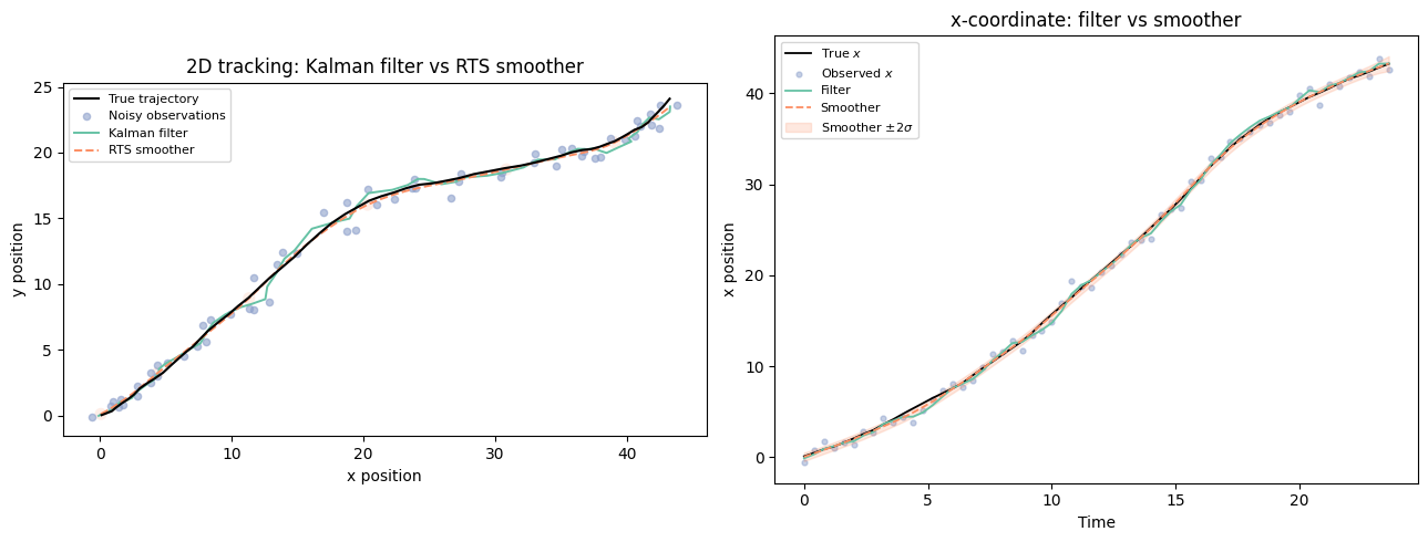
# ── 2D tracking demo: constant-velocity model ─────────────────────────────────
# State: z = [x, y, vx, vy]   (position + velocity in 2D)
# Observation: x = [px, py]   (noisy position)
import numpy as np

dt = 0.4
T_demo = 60
torch.manual_seed(42)

# Model parameters
A = torch.eye(4)
A[0, 2] = dt
A[1, 3] = dt

b      = torch.zeros(4)
Q      = torch.diag(torch.tensor([1e-4, 1e-4, 0.05, 0.05]))

C      = torch.zeros(2, 4)
C[0, 0] = 1.0
C[1, 1] = 1.0
d      = torch.zeros(2)
R      = 0.4 * torch.eye(2)

mu0    = torch.tensor([0.0, 0.0, 0.8, 0.3])
Sigma0 = 0.1 * torch.eye(4)

# ── Simulate from the model ───────────────────────────────────────────────────
z_true = torch.zeros(T_demo, 4)
y_obs  = torch.zeros(T_demo, 2)

z_true[0] = dist.MultivariateNormal(mu0, Sigma0).sample()
y_obs[0]  = dist.MultivariateNormal(C @ z_true[0] + d, R).sample()
for t in range(1, T_demo):
    z_true[t] = dist.MultivariateNormal(A @ z_true[t-1] + b, Q).sample()
    y_obs[t]  = dist.MultivariateNormal(C @ z_true[t] + d, R).sample()

# ── Run filter and smoother ───────────────────────────────────────────────────
filt_mu, filt_S, pred_mu, pred_S, log_ml = kalman_filter(
    y_obs, A, b, Q, C, d, R, mu0, Sigma0)
smooth_mu, smooth_S = rts_smoother(A, filt_mu, filt_S, pred_mu, pred_S)

print(f"Log marginal likelihood: {log_ml:.2f}")

# ── Helper: draw a 2-sigma covariance ellipse (numpy-based) ──────────────────
def cov_ellipse(ax, mean_np, cov_np, n_std=2.0, **kwargs):
    from matplotlib.patches import Ellipse
    eigenvalues, eigenvectors = np.linalg.eigh(cov_np)
    angle = np.degrees(np.arctan2(eigenvectors[1, -1], eigenvectors[0, -1]))
    width, height = 2 * n_std * np.sqrt(eigenvalues)
    ell = Ellipse(xy=mean_np, width=width, height=height, angle=angle, **kwargs)
    ax.add_patch(ell)

# ── Plot ──────────────────────────────────────────────────────────────────────
fig, axes = plt.subplots(1, 2, figsize=(13, 5))

# ── Panel 1: 2D trajectories ──────────────────────────────────────────────────
ax = axes[0]
ax.plot(z_true[:, 0], z_true[:, 1], 'k-', lw=1.5, zorder=4, label='True trajectory')
ax.scatter(y_obs[:, 0], y_obs[:, 1], s=20, alpha=0.6,
           color=palette[2], zorder=3, label='Noisy observations')
ax.plot(filt_mu[:, 0], filt_mu[:, 1],
        color=palette[0], lw=1.4, zorder=3, label='Kalman filter')
ax.plot(smooth_mu[:, 0], smooth_mu[:, 1],
        color=palette[1], lw=1.4, linestyle='--', zorder=3, label='RTS smoother')

for t in range(0, T_demo, 10):
    cov_np   = smooth_S[t, :2, :2].detach().numpy()
    mean_np  = smooth_mu[t, :2].detach().numpy()
    cov_ellipse(ax, mean_np, cov_np,
                n_std=2, facecolor=palette[1], alpha=0.15, edgecolor='none')

ax.set_title('2D tracking: Kalman filter vs RTS smoother')
ax.set_xlabel('x position')
ax.set_ylabel('y position')
ax.legend(fontsize=8)
ax.set_aspect('equal')

# ── Panel 2: x-coordinate time series ─────────────────────────────────────────
ax = axes[1]
t_vals = dt * np.arange(T_demo)

ax.plot(t_vals, z_true[:, 0].numpy(), 'k-', lw=1.3, label='True $x$')
ax.scatter(t_vals, y_obs[:, 0].numpy(), s=12, alpha=0.5,
           color=palette[2], label='Observed $x$')
ax.plot(t_vals, filt_mu[:, 0].numpy(), color=palette[0], lw=1.3, label='Filter')
ax.plot(t_vals, smooth_mu[:, 0].numpy(), color=palette[1],
        lw=1.3, linestyle='--', label='Smoother')

sig_x = smooth_S[:, 0, 0].sqrt().numpy()
ax.fill_between(t_vals,
                smooth_mu[:, 0].numpy() - 2 * sig_x,
                smooth_mu[:, 0].numpy() + 2 * sig_x,
                alpha=0.2, color=palette[1], label='Smoother $\pm 2\sigma$')

ax.set_title('x-coordinate: filter vs smoother')
ax.set_xlabel('Time')
ax.set_ylabel('x position')
ax.legend(fontsize=8)

plt.tight_layout()
plt.show()

<>:93: SyntaxWarning: invalid escape sequence '\p'
<>:93: SyntaxWarning: invalid escape sequence '\p'
/tmp/ipykernel_2744/2116936060.py:93: SyntaxWarning: invalid escape sequence '\p'
  alpha=0.2, color=palette[1], label='Smoother $\pm 2\sigma$')

Log marginal likelihood: -148.77

Conclusion¶

Algorithm	Pass	Output	Cost
Kalman filter	Forward	$p(\mathbf{z}_t \mid \mathbf{x}_{1:t})$	$O(T D_z^3)$
RTS smoother	Backward	$p(\mathbf{z}_t \mid \mathbf{x}_{1:T})$	$O(T D_z^3)$

The Kalman filter and RTS smoother are the exact continuous-state analogues of the discrete forward-backward algorithm: they exploit the Markov structure to compute marginals in linear time.

Learning. Given the smoothed marginals, the EM M-step for LDS parameters has closed forms analogous to the mixture model case. The sufficient statistics are $\mathbb{E}[\mathbf{z}_t]$ , $\mathbb{E}[\mathbf{z}_t \mathbf{z}_t^\top]$ , and $\mathbb{E}[\mathbf{z}_t \mathbf{z}_{t-1}^\top]$ , all of which follow from the smoothed means and covariances. This is sometimes called the EM algorithm for LDS or the Shumway-Stoffer algorithm Shumway & Stoffer, 2000.