Switching Linear Dynamical Systems

Both HMMs and LDS capture temporal dynamics in latent-variable models, but each has a fundamental limitation. An HMM assumes the hidden state is discrete — it can represent switching behaviour but cannot track smoothly evolving continuous quantities. An LDS assumes a single linear Gaussian regime — it can track smooth continuous dynamics but cannot represent abrupt regime changes.

A switching linear dynamical system (SLDS) combines both: a discrete chain $z_{1:T}$ that selects which linear regime is active at each step, and a continuous chain $\mbx_{1:T}$ whose dynamics depend on that regime. The model can represent a system that moves smoothly within each regime but switches sharply between them.

Topics covered:

The SLDS generative model
Why exact EM is intractable: forward messages are exponential mixtures
Structured mean-field variational inference: alternating HMM and Kalman updates
Recurrent SLDS and Variational Laplace EM

import torch
import torch.distributions as dist
import matplotlib.pyplot as plt
import matplotlib.patches as mpatches
import numpy as np

palette = list(plt.cm.tab10.colors)
torch.manual_seed(305)

<torch._C.Generator at 0x7f8758bd79f0>

The SLDS Generative Model¶

An SLDS has three layers of latent structure:

Layer	Variable	Role
Discrete chain	$z_t \in \{1,\ldots,K\}$	Which dynamical regime is active
Continuous chain	$\mbx_t \in \reals^{D_x}$	Continuously evolving latent state
Observations	$\mby_t \in \reals^{D_y}$	Noisy linear readout of $\mbx_t$

The joint distribution is:

p(z_{1:T}, \mbx_{1:T}, \mby_{1:T}) = p(z_1)\,p(\mbx_1 \mid z_1) \prod_{t=2}^T p(z_t \mid z_{t-1})\,p(\mbx_t \mid \mbx_{t-1}, z_t) \prod_{t=1}^T p(\mby_t \mid \mbx_t).

(1)

Each factor is defined as follows.

Discrete chain (HMM). The discrete states follow a Markov chain with initial distribution $\mbpi_0$ and transition matrix $\mbP$ :

z_1 \sim \mathrm{Cat}(\mbpi_0), \qquad z_t \mid z_{t-1} \sim \mathrm{Cat}(\mbP_{z_{t-1},\cdot}).

(2)

Continuous chain (switched LDS). Given the discrete state, the continuous state evolves as a linear Gaussian with regime-specific parameters:

\mbx_1 \mid z_1 \sim \cN(\mbb_{z_1}, \mbQ_{z_1}), \qquad \mbx_t \mid \mbx_{t-1}, z_t \sim \cN(\mbA_{z_t}\mbx_{t-1} + \mbb_{z_t},\; \mbQ_{z_t}).

(3)

Emissions (shared). Observations are a noisy linear readout of the continuous state, shared across all regimes:

\mby_t \mid \mbx_t \sim \cN(\mbC\mbx_t + \mbd,\; \mbR).

(4)

The parameters are $\theta = \{\mbpi_0, \mbP, \{\mbA_k, \mbb_k, \mbQ_k\}_{k=1}^K, \mbC, \mbd, \mbR\}$ .

Exact Inference is Intractable¶

For EM, the E-step requires computing the posterior $p(z_{1:T}, \mbx_{1:T} \mid \mby_{1:T})$ . The natural approach is to run a forward pass over the hybrid state $h_t = (z_t, \mbx_t)$ , maintaining the joint message

\alpha_t(k, \mbx) \propto p(z_t = k,\; \mbx_t = \mbx,\; \mby_{1:t}).

(5)

At $t=1$ this is a mixture of $K$ Gaussians (one per initial discrete state). Propagating one step, for each $(k', \mbx_{t+1})$ :

\alpha_{t+1}(k', \mbx_{t+1}) = \sum_{k=1}^K P_{kk'} \int \cN(\mbx_{t+1};\; \mbA_{k'}\mbx_t + \mbb_{k'},\, \mbQ_{k'}) \;\alpha_t(k, \mbx_t)\; d\mbx_t.

(6)

Each of the $K$ existing Gaussian components at time $t$ spawns $K$ new components at time $t+1$ (one for each incoming discrete state). The number of components multiplies at each step:

\text{components at time }T = K^T.

(7)

For $K=3$ and $T=100$ , this is $3^{100} \approx 5 \times 10^{47}$ — clearly intractable. We need an approximation.

Approximate Message Passing: Gaussian Sum Filter¶

Rather than abandoning message passing altogether, one family of approximations attempts to keep the forward pass tractable by maintaining a bounded-size mixture at each step. The idea is simple: the exact forward message after $t$ steps is a mixture of $K^t$ Gaussians; instead, we maintain only $M$ Gaussian components per discrete state (for some small fixed $M$ ), and after each propagation step we collapse the expanded mixture back to $M$ components. This is the Gaussian Sum Filter (GSF) Barber, 2012, Ch.~25.

The Gaussian Sum Filter¶

Represent the filtered distribution as a finite mixture, separately for each discrete state $k$ :

q(\mbx_t, z_t = k \mid \mby_{1:t}) = q(z_t=k \mid \mby_{1:t})\;\sum_{m=1}^M w_t(m, k)\;\cN(\mbx_t;\; \mbf_t(m,k),\; \mbF_t(m,k)),

(8)

where $\sum_m w_t(m,k) = 1$ for each $k$ . The full filtered distribution is a mixture of $KM$ Gaussians in total.

Propagation. Given the $KM$ -component approximation at time $t$ , one forward step produces a $KM \cdot K = K^2 M$ component mixture at time $t+1$ : for each incoming component $(m, k)$ and each new discrete state $k'$ , run a standard Kalman predict-update step with dynamics $(\mbA_{k'}, \mbb_{k'}, \mbQ_{k'})$ and observation $\mby_{t+1}$ :

q(\mbx_{t+1} \mid z_{t+1}=k', z_t=k, \text{comp.}\,m, \mby_{1:t+1}) = \cN(\mbx_{t+1};\; \mbmu_{t+1}^{k',k,m},\; \mbSigma_{t+1}^{k',k,m}).

(9)

The weight of this component is proportional to:

P_{kk'}\cdot p(\mby_{t+1} \mid z_{t+1}=k', z_t=k, \text{comp.}\,m, \mby_{1:t}) \cdot w_t(m,k)\cdot q(z_t=k \mid \mby_{1:t}),

(10)

where $p(\mby_{t+1} \mid \cdots)$ is the Gaussian predictive likelihood from the Kalman step.

Collapse. To keep the mixture bounded at $M$ components per discrete state, merge the $K \cdot M$ components for each $k'$ back to $M$ . The simplest approach retains the $M-1$ highest-weight components and merges the remaining ones into a single Gaussian by moment matching: given components with weights $\{p_j\}$ and parameters $\{\mbmu_j, \mbSigma_j\}$ , compute

\bar\mbmu = \sum_j p_j \mbmu_j, \qquad \bar\mbSigma = \sum_j p_j\bigl(\mbSigma_j + (\mbmu_j - \bar\mbmu)(\mbmu_j - \bar\mbmu)^\top\bigr).

(11)

This completes one forward step of the Gaussian Sum Filter.

The $M = 1$ Special Case¶

With $M = 1$ (a single Gaussian per discrete state), the filter collapses to the single-component approximation, sometimes called the Gaussian Sum Filter with moment matching or, in the engineering literature, the Interacting Multiple Models (IMM) filter. At each step the continuous distribution conditioned on each discrete state is approximated by a single Gaussian:

q(\mbx_t \mid z_t = k, \mby_{1:t}) \approx \cN(\mbx_t;\; \mbmu_t^k,\; \mbSigma_t^k).

(12)

The marginal over the continuous state is then a $K$ -component mixture:

q(\mbx_t \mid \mby_{1:t}) = \sum_{k=1}^K q(z_t=k \mid \mby_{1:t})\;\cN(\mbx_t;\; \mbmu_t^k,\; \mbSigma_t^k).

(13)

This is tractable at every step: $O(TK^2 D_x^3)$ total, since each of the $K$ Kalman steps costs $O(D_x^3)$ and there are $K^2$ component pairs.

Approximate Smoothing¶

The backward (smoothing) pass requires analogous approximations. One popular method is the Expectation Correction (EC) smoother Barber, 2012, which approximates $p(\mbx_{t+1} \mid z_t, z_{t+1}, \mby_{1:T}) \approx p(\mbx_{t+1} \mid z_{t+1}, \mby_{1:T})$ , dropping the dependence on the current discrete state. This allows an RTS-style backward recursion for each discrete state, followed by moment-matching to collapse the resulting mixture.

A simpler alternative is Generalised Pseudo-Bayes (GPB) smoothing, which approximates $p(z_t \mid z_{t+1}, \mby_{1:T}) \approx p(z_t \mid z_{t+1}, \mby_{1:t})$ and runs the HMM backward pass independently of the continuous backward recursion. GPB is computationally cheaper but discards future information passed through the continuous variables.

Structured Mean-Field Variational Inference¶

The Mean-Field Family¶

The structured mean-field approximation breaks the dependence between the two chains while preserving the Markov structure within each:

q(z_{1:T}, \mbx_{1:T}) = q(z_{1:T}) \cdot q(\mbx_{1:T}).

(14)

We require that $q(z_{1:T})$ factorises as an HMM-type chain and $q(\mbx_{1:T})$ factorises as an LDS-type chain. We find the best $q$ by minimising the KL divergence:

q^* = \operatorname*{arg\,min}_{q} \;D_\mathrm{KL}\bigl(q(z_{1:T}, \mbx_{1:T}) \,\|\, p(z_{1:T}, \mbx_{1:T} \mid \mby_{1:T})\bigr).

(15)

By the CAVI theorem (CAVI chapter), the optimal update for each factor, holding the other fixed, is:

\log q^*(z_{1:T}) = \E_{q(\mbx)}\bigl[\log p(z_{1:T}, \mbx_{1:T}, \mby_{1:T})\bigr] + \text{const.}

(16)

CAVI Update for $q(z_{1:T})$ ¶

Collecting terms that involve $z_{1:T}$ :

\log q(z_{1:T}) = \log p(z_1) + \sum_{t=2}^T \log P_{z_{t-1},z_t} + \sum_{t=1}^T \ell_t(z_t) + \text{const},

(17)

where the expected log-likelihoods under $q(\mbx)$ are:

\ell_t(k) = \E_{q(\mbx)}\!\bigl[\log p(\mbx_t \mid \mbx_{t-1}, z_t=k)\bigr] = \E_{q(\mbx)}\!\bigl[\log \cN(\mbx_t;\; \mbA_k\mbx_{t-1}+\mbb_k,\, \mbQ_k)\bigr].

(18)

This has exactly the structure of an HMM with log-likelihoods $\{\ell_t(k)\}$ in place of observation log-likelihoods.

$q(z)$ update: run HMM forward-backward with transition matrix $\mbP$ and log-likelihoods $\{\ell_t(k)\}$ to obtain the marginals $\gamma_t(k) = q(z_t = k)$ and pairwise marginals $\xi_t(j,k) = q(z_{t-1}=j, z_t=k)$ .

Computing $\ell_t(k)$ . Expanding the Gaussian log-likelihood, the expectation requires only three smoother moments: $\E_q[\mbx_t]$ , $\E_q[\mbx_t\mbx_t^\top]$ , and $\E_q[\mbx_t\mbx_{t-1}^\top]$ . All three are available from the RTS smoother run in the previous $q(\mbx)$ update.

CAVI Update for $q(\mbx_{1:T})$ ¶

Collecting terms that involve $\mbx_{1:T}$ :

\log q(\mbx_{1:T}) \propto \E_{q(z)}\!\left[\sum_{t=2}^T \log p(\mbx_t \mid \mbx_{t-1}, z_t) + \sum_{t=1}^T \log p(\mby_t \mid \mbx_t)\right].

(19)

The emission terms do not depend on $z_t$ . The dynamics terms average over $z_t$ using the marginals $\gamma_t(k) = q(z_t = k)$ :

\E_{q(z)}\bigl[\log p(\mbx_t \mid \mbx_{t-1}, z_t)\bigr] = \sum_{k=1}^K \gamma_t(k)\,\log \cN(\mbx_t;\; \mbA_k\mbx_{t-1}+\mbb_k,\, \mbQ_k).

(20)

With a shared noise covariance $\mbQ_k = \mbQ$ (same for all $k$ ), this sum of log-Gaussians is itself a log-Gaussian with effective dynamics:

\bar\mbA_t = \sum_{k=1}^K \gamma_t(k)\,\mbA_k, \qquad \bar\mbb_t = \sum_{k=1}^K \gamma_t(k)\,\mbb_k.

(21)

$q(\mbx)$ update: run Kalman filter + RTS smoother with time-varying dynamics $(\bar\mbA_t, \bar\mbb_t, \mbQ)$ and fixed emissions $(\mbC, \mbd, \mbR)$ to obtain the smoothed moments $\E_q[\mbx_t]$ , $\E_q[\mbx_t\mbx_t^\top]$ , $\E_q[\mbx_t\mbx_{t-1}^\top]$ .

Full Variational EM Algorithm¶

Combining the two CAVI updates with an M-step gives the full algorithm.

Initialize: $\gamma_t(k) \leftarrow 1/K$ for all $t, k$ .

Repeat until convergence:

(E.1) Compute expected log-likelihoods: for each $t = 1,\ldots,T$ and $k = 1,\ldots,K$ ,

\ell_t(k) = -\tfrac{D_x}{2}\log(2\pi) - \tfrac{1}{2}\log|\mbQ_k| - \tfrac{1}{2}\,\E_q\!\left[\|\mbQ_k^{-1/2}(\mbx_t - \mbA_k\mbx_{t-1} - \mbb_k)\|^2\right].

(22)

(E.2) Update $q(z_{1:T})$ : run HMM forward-backward with $\{\ell_t(k)\}$ to obtain $\gamma_t(k)$ and $\xi_t(j,k)$ .

(E.3) Update $q(\mbx_{1:T})$ : run Kalman filter + RTS smoother with soft-averaged dynamics $\bar\mbA_t = \sum_k \gamma_t(k)\mbA_k$ and $\bar\mbb_t = \sum_k \gamma_t(k)\mbb_k$ to obtain $\E_q[\mbx_t]$ , $\E_q[\mbx_t\mbx_t^\top]$ , $\E_q[\mbx_t\mbx_{t-1}^\top]$ .

(M-step) Update parameters using the expected sufficient statistics:

\hat{P}_{jk} \propto \sum_{t=2}^T \xi_t(j,k), \qquad \hat{\mbA}_k = \left(\sum_{t=2}^T \gamma_t(k)\,\E_q[\mbx_t\mbx_{t-1}^\top]\right) \left(\sum_{t=2}^T \gamma_t(k)\,\E_q[\mbx_{t-1}\mbx_{t-1}^\top]\right)^{-1}.

(23)

Recurrent SLDS¶

Motivation and Model¶

In the standard SLDS, the transition $p(z_t \mid z_{t-1})$ depends only on the previous discrete state — the continuous state $\mbx_{t-1}$ has no influence on which regime is active next. This is a significant limitation: in many physical systems, regime changes are triggered by crossing a threshold in the continuous state (e.g. a neuron switching firing mode when membrane potential crosses a threshold; a locomotor system changing gait when speed exceeds a threshold).

The Recurrent SLDS (rSLDS) Linderman et al., 2017 adds a direct dependence of the discrete transition on the previous continuous state $\mbx_{t-1}$ :

p(z_t = k \mid z_{t-1}, \mbx_{t-1}) \propto \exp\!\bigl(\mbw_k^\top \mbx_{t-1} + b_k\bigr).

(24)

The weight vectors $\mbw_k \in \reals^{D_x}$ define hyperplanes that partition the continuous state space: the model transitions to regime $k$ when $\mbx_{t-1}$ lies in the region where $\mbw_k^\top\mbx_{t-1}$ is largest. This couples the two chains far more tightly: the discrete state depends on the continuous state, and the continuous dynamics depend on the discrete state.

The rSLDS has been applied to neural population dynamics, where the continuous state represents a latent neural trajectory and the discrete state represents distinct decision-making phases Zoltowski et al., 2020. The recurrent transitions allow the model to learn where in latent space each phase applies, rather than treating phase transitions as random.

Challenge for inference. The expected log-likelihoods $\ell_t(k)$ for the $q(z)$ update now include a softmax log-probability that is nonlinear in $\mbx_{t-1}$ :

\ell_t(k) = \E_{q(\mbx)}\!\bigl[\log p(z_t=k \mid z_{t-1}, \mbx_{t-1}) + \log p(\mbx_t \mid \mbx_{t-1}, z_t=k)\bigr].

(25)

The nonlinear softmax term means the $q(\mbx)$ update is no longer a standard Kalman pass. This motivates the Variational Laplace EM algorithm described next.

Variational Laplace EM¶

Key idea Zoltowski et al., 2020. Rather than trying to compute $q(\mbx_{1:T})$ in closed form, approximate it with a Laplace approximation around the MAP estimate:

q(\mbx_{1:T} \mid z_{1:T}) \approx \cN\!\bigl(\hat\mbx_z,\; \mbH_z^{-1}\bigr),

(26)

where

\hat\mbx_z = \operatorname*{arg\,max}_{\mbx_{1:T}}\; \log p(\mbx_{1:T} \mid z_{1:T}, \mby_{1:T};\,\theta),

(27)

\mbH_z = -\nabla^2_{\mbx_{1:T}} \log p(\mbx_{1:T} \mid z_{1:T}, \mby_{1:T};\,\theta)\Big|_{\mbx_{1:T}=\hat\mbx_z}.

(28)

Block-tridiagonal structure. The Markov structure of the model means $\mbx_t$ is coupled to $\mbx_{t-1}$ and $\mbx_{t+1}$ in the log-posterior but not to more distant time steps. Consequently $\mbH_z$ is block-tridiagonal with blocks of size $D_x \times D_x$ . The MAP solve (Newton’s method) and the Hessian inversion both cost $O(T D_x^3)$ — the same as a Kalman smoother pass.

Reduction to Kalman smoother. For the standard SLDS with linear Gaussian dynamics and a fixed discrete sequence, the log-posterior is quadratic in $\mbx_{1:T}$ , so the Laplace approximation is exact: $\hat\mbx_z$ is the RTS smoother mean and $\mbH_z^{-1}$ is the RTS smoother covariance.

Algorithm. The variational Laplace EM algorithm Zoltowski et al., 2020 alternates the same three steps as structured mean-field, but replaces the Kalman smoother in E.3 with a MAP solve:

(E.1) Find MAP $\hat\mbx$ by Newton’s method on $\log p(\mbx \mid z, \mby)$ ; compute block-tridiagonal $\mbH^{-1}$ from the Hessian at $\hat\mbx$ .

(E.2) Compute $\ell_t(k)$ using moments from $\hat\mbx$ and $\mbH^{-1}$ (including the nonlinear softmax log-probability).

(E.3) Update $q(z_{1:T})$ : run HMM forward-backward with $\{\ell_t(k)\}$ .

Implementation: Structured Mean-Field VI¶

We implement the structured mean-field algorithm for an SLDS with shared emission parameters and shared noise covariance $\mbQ$ .

Helper: Kalman Filter and RTS Smoother¶

We need a Kalman filter that accepts time-varying dynamics $\bar\mbA_t, \bar\mbb_t$ (the soft-averaged matrices from $\gamma_t(k)$ ), and an RTS smoother that also returns the lagged cross-covariances $\E_q[\mbx_t\mbx_{t-1}^\top]$ needed to evaluate $\ell_t(k)$ .

def kalman_filter_tvd(y, A_seq, b_seq, Q, C, d, R, mu0, Sigma0):
    """Kalman filter with time-varying dynamics.

    Args:
        y:      (T, Dy)
        A_seq:  (T, Dx, Dx)  time-varying dynamics; A_seq[t] used for step t->t+1
        b_seq:  (T, Dx)
        Q:      (Dx, Dx)     shared dynamics noise covariance
        C:      (Dy, Dx)
        d:      (Dy,)
        R:      (Dy, Dy)
        mu0:    (Dx,)
        Sigma0: (Dx, Dx)
    Returns:
        μ_filt  (T, Dx), Σ_filt (T, Dx, Dx)
        μ_pred  (T, Dx), Σ_pred (T, Dx, Dx)
        G_gains (T-1, Dx, Dx)  smoother gains (computed here for reuse)
        log_ml  scalar
    """
    T, Dy = y.shape
    Dx = mu0.shape[0]
    I = torch.eye(Dx)

    μ_filt = torch.zeros(T, Dx)
    Σ_filt = torch.zeros(T, Dx, Dx)
    μ_pred = torch.zeros(T, Dx)
    Σ_pred = torch.zeros(T, Dx, Dx)
    log_ml = 0.0

    μ = mu0.clone()
    Σ = Sigma0.clone()

    for t in range(T):
        μ_pred[t] = μ
        Σ_pred[t] = Σ

        # Update
        innov = y[t] - C @ μ - d
        S = C @ Σ @ C.T + R
        K = Σ @ C.T @ torch.linalg.solve(S, torch.eye(Dy))
        μ = μ + K @ innov
        Σ = (I - K @ C) @ Σ
        log_ml += dist.MultivariateNormal(C @ μ_pred[t] + d, S).log_prob(y[t])

        μ_filt[t] = μ
        Σ_filt[t] = Σ

        # Predict (not needed after last step)
        if t < T - 1:
            A_t = A_seq[t]
            μ = A_t @ μ + b_seq[t]
            Σ = A_t @ Σ @ A_t.T + Q

    return μ_filt, Σ_filt, μ_pred, Σ_pred, log_ml


def rts_smoother_tvd(A_seq, μ_filt, Σ_filt, μ_pred, Σ_pred):
    """RTS smoother with time-varying dynamics.

    Returns smoothed means, covariances, smoother gains, and lagged
    cross-covariances Cov[x_t, x_{t-1} | y_{1:T}] = Σ_{t|T} G_{t-1}^T.
    """
    T, Dx = μ_filt.shape
    μ_smooth = μ_filt.clone()
    Σ_smooth = Σ_filt.clone()
    G_gains = torch.zeros(T - 1, Dx, Dx)
    cross_covs = torch.zeros(T - 1, Dx, Dx)  # Cov[x_t, x_{t-1}], indexed by t

    for t in range(T - 2, -1, -1):
        A_t = A_seq[t]
        G = Σ_filt[t] @ A_t.T @ torch.linalg.solve(Σ_pred[t + 1], torch.eye(Dx))
        G_gains[t] = G
        μ_smooth[t] = μ_filt[t] + G @ (μ_smooth[t + 1] - μ_pred[t + 1])
        Σ_smooth[t] = Σ_filt[t] + G @ (Σ_smooth[t + 1] - Σ_pred[t + 1]) @ G.T
        # Cov[x_{t+1}, x_t | y_{1:T}] = Σ_{t+1|T} G_t^T
        cross_covs[t] = Σ_smooth[t + 1] @ G.T

    return μ_smooth, Σ_smooth, G_gains, cross_covs

# ── Expected log-likelihoods ℓ_t(k) ──────────────────────────────────────────

def compute_ell(μ_s, Σ_s, cross_covs, A_list, b_list, Q):
    """Compute ℓ_t(k) = E_{q(x)}[log p(x_t | x_{t-1}, z_t=k)] for t=1,...,T-1.

    Args:
        μ_s:        (T, Dx)      smoothed means
        Σ_s:        (T, Dx, Dx)  smoothed covariances
        cross_covs: (T-1, Dx, Dx) cross_covs[t] = Cov[x_{t+1}, x_t | y_{1:T}]
        A_list:     list of K (Dx, Dx) dynamics matrices
        b_list:     list of K (Dx,) biases
        Q:          (Dx, Dx)
    Returns:
        ell: (T-1, K)  log-likelihoods for t=1,...,T-1
             (t=0 not included since x_t|x_{t-1} only defined for t>=1)
    """
    T, Dx = μ_s.shape
    K = len(A_list)
    Q_inv = torch.linalg.inv(Q)
    log_det_Q = torch.logdet(Q)
    const = -0.5 * (Dx * torch.log(torch.tensor(2 * torch.pi)) + log_det_Q)

    # Second moments
    E_xt_xt = Σ_s[1:] + μ_s[1:].unsqueeze(2) * μ_s[1:].unsqueeze(1)       # (T-1,Dx,Dx)
    E_xp_xp = Σ_s[:-1] + μ_s[:-1].unsqueeze(2) * μ_s[:-1].unsqueeze(1)    # (T-1,Dx,Dx)
    # cross_covs[t] = Cov[x_{t+1},x_t] so E[x_{t+1} x_t^T] = cross_covs[t] + mu[t+1] mu[t]^T
    E_xt_xp = cross_covs + μ_s[1:].unsqueeze(2) * μ_s[:-1].unsqueeze(1)    # (T-1,Dx,Dx)

    ell = torch.zeros(T - 1, K)
    for k, (A_k, b_k) in enumerate(zip(A_list, b_list)):
        # E[||Q^{-1/2}(x_t - A_k x_{t-1} - b_k)||^2]
        # = Tr[Q_inv @ (E[x_t x_t^T] - E[x_t x_{t-1}^T] A_k^T - b_k E[x_t]^T
        #               - A_k E[x_{t-1} x_t^T] + A_k E[x_{t-1} x_{t-1}^T] A_k^T
        #               + A_k E[x_{t-1}] b_k^T - b_k E[x_{t-1}]^T A_k^T + b_k b_k^T)]
        # Combine into M_t for each t:
        M = (E_xt_xt
             - E_xt_xp @ A_k.T                                          # -E[x_t x_{t-1}^T] A_k^T
             - μ_s[1:].unsqueeze(2) * b_k.unsqueeze(0).unsqueeze(0)    # -b_k E[x_t]^T  (outer)
             - A_k @ E_xt_xp.transpose(1, 2)                           # -A_k E[x_{t-1} x_t^T]
             + A_k @ E_xp_xp @ A_k.T                                   # A_k E[x_{t-1}^2] A_k^T
             + (A_k @ μ_s[:-1].unsqueeze(2)) * b_k.unsqueeze(0).unsqueeze(0)  # A_k mu b_k^T
             - b_k.unsqueeze(1) * (A_k @ μ_s[:-1].unsqueeze(2)).squeeze(2).unsqueeze(1)  # b_k mu^T A_k^T
             + b_k.unsqueeze(1) * b_k.unsqueeze(0))                    # b_k b_k^T

        ell[:, k] = const - 0.5 * torch.einsum('tij,ji->t', M, Q_inv)

    return ell  # (T-1, K)


# ── HMM forward-backward (reusing the convention from ch. 04_01) ──────────────

def hmm_forward(log_pi0, log_P, log_ell):
    """Normalized forward messages. Returns log_alphas (T, K) and log_norms (T,).

    Convention: log_alphas[t, k] = log p(z_t=k | y_{1:t-1})  (predictive).
    log_ell[t, k] = log p(x_t | x_{t-1}, z_t=k)  (ell_t(k) from compute_ell,
    extended with a zero column at t=0 since z_1 has no dynamics likelihood).
    """
    T, K = log_ell.shape
    log_alphas = torch.zeros(T, K)
    log_norms = torch.zeros(T)

    log_alphas[0] = log_pi0 - torch.logsumexp(log_pi0, 0)
    log_norms[0] = torch.logsumexp(log_alphas[0] + log_ell[0], 0)

    for t in range(1, T):
        log_joint = log_alphas[t - 1] + log_ell[t - 1]
        log_alpha_t = torch.logsumexp(log_joint[:, None] + log_P, 0)
        log_alphas[t] = log_alpha_t - torch.logsumexp(log_alpha_t, 0)
        log_norms[t] = torch.logsumexp(log_alphas[t] + log_ell[t], 0)

    return log_alphas, log_norms


def hmm_backward(log_P, log_ell):
    T, K = log_ell.shape
    log_betas = torch.zeros(T, K)
    for t in range(T - 2, -1, -1):
        log_joint = log_ell[t + 1] + log_betas[t + 1]
        log_beta_t = torch.logsumexp(log_P + log_joint[None, :], 1)
        log_betas[t] = log_beta_t - torch.logsumexp(log_beta_t, 0)
    return log_betas


def hmm_marginals(log_alphas, log_betas, log_ell):
    log_gamma = log_alphas + log_ell + log_betas
    log_gamma -= torch.logsumexp(log_gamma, 1, keepdim=True)
    return log_gamma.exp()  # (T, K)


def hmm_pair_marginals(log_alphas, log_betas, log_ell, log_P):
    T, K = log_alphas.shape
    log_xi = (log_alphas[:-1, :, None]
              + log_ell[:-1, :, None]
              + log_P[None]
              + log_ell[1:, None, :]
              + log_betas[1:, None, :])
    log_xi -= torch.logsumexp(log_xi.reshape(T - 1, -1), 1).reshape(T - 1, 1, 1)
    return log_xi.exp()  # (T-1, K, K)

# ── Structured mean-field variational EM ─────────────────────────────────────

def slds_mean_field_em(
    y,
    A_list, b_list, Q,
    C, d, R,
    pi0, P,
    mu0, Sigma0,
    num_iters=30,
):
    """Structured mean-field variational EM for SLDS.

    Parameters are assumed fixed (E-step only; M-step not implemented here).

    Args:
        y:       (T, Dy)
        A_list:  list of K (Dx, Dx)
        b_list:  list of K (Dx,)
        Q:       (Dx, Dx) shared dynamics noise
        C:       (Dy, Dx)
        d:       (Dy,)
        R:       (Dy, Dy)
        pi0:     (K,) initial discrete distribution
        P:       (K, K) transition matrix
        mu0:     (Dx,) initial continuous mean
        Sigma0:  (Dx, Dx)
    Returns:
        γ:       (T, K) posterior marginals q(z_t=k)
        μ_s:     (T, Dx) smoothed continuous means
        Σ_s:     (T, Dx, Dx) smoothed continuous covariances
    """
    T, Dy = y.shape
    K = len(A_list)
    Dx = A_list[0].shape[0]
    A_stack = torch.stack(A_list)  # (K, Dx, Dx)
    b_stack = torch.stack(b_list)  # (K, Dx)

    log_P = P.log()
    log_pi0 = pi0.log()

    # Initialize γ uniformly
    γ = torch.full((T, K), 1.0 / K)

    μ_s = torch.zeros(T, Dx)
    Σ_s = torch.zeros(T, Dx, Dx)
    cross_covs = torch.zeros(T - 1, Dx, Dx)

    for _ in range(num_iters):
        # ── E.3: update q(x) with soft-averaged dynamics ──────────────────
        A_eff = torch.einsum('tk,kij->tij', γ, A_stack)   # (T, Dx, Dx)
        b_eff = torch.einsum('tk,ki->ti', γ, b_stack)     # (T, Dx)
        μ_filt, Σ_filt, μ_pred, Σ_pred, _ = kalman_filter_tvd(
            y, A_eff, b_eff, Q, C, d, R, mu0, Sigma0)
        μ_s, Σ_s, _, cross_covs = rts_smoother_tvd(
            A_eff, μ_filt, Σ_filt, μ_pred, Σ_pred)

        # ── E.1: compute ℓ_t(k) ──────────────────────────────────────────
        ell = compute_ell(μ_s, Σ_s, cross_covs, A_list, b_list, Q)  # (T-1, K)

        # Pad to (T, K): t=0 has no dynamics likelihood so set to 0
        log_ell = torch.cat([torch.zeros(1, K), ell], dim=0)  # (T, K)

        # ── E.2: update q(z) via HMM forward-backward ────────────────────
        log_alphas, _ = hmm_forward(log_pi0, log_P, log_ell)
        log_betas = hmm_backward(log_P, log_ell)
        γ = hmm_marginals(log_alphas, log_betas, log_ell)

    return γ, μ_s, Σ_s

# ── Simulate from a two-regime SLDS ──────────────────────────────────────────
# Regime 1: slow clockwise rotation (stable spiral in)
# Regime 2: fast counter-clockwise rotation (stable spiral out, then in)
torch.manual_seed(305)

K, Dx, Dy = 2, 2, 2
T = 150

# Regime 1: slowly decaying clockwise rotation
θ1 = torch.tensor(0.15)   # rotation angle
r1 = 0.97
A1 = r1 * torch.tensor([[torch.cos(θ1), -torch.sin(θ1)],
                         [torch.sin(θ1),  torch.cos(θ1)]])
b1 = torch.zeros(Dx)

# Regime 2: faster counter-clockwise rotation with slight expansion
θ2 = torch.tensor(-0.35)
r2 = 0.94
A2 = r2 * torch.tensor([[torch.cos(θ2), -torch.sin(θ2)],
                         [torch.sin(θ2),  torch.cos(θ2)]])
b2 = torch.zeros(Dx)

Q = 0.03 * torch.eye(Dx)
C = torch.eye(Dy, Dx)
d = torch.zeros(Dy)
R = 0.2 * torch.eye(Dy)

pi0 = torch.tensor([0.8, 0.2])
P = torch.tensor([[0.95, 0.05],
                  [0.10, 0.90]])

mu0 = torch.tensor([2.0, 0.0])
Sigma0 = 0.1 * torch.eye(Dx)

# Simulate
z_true = torch.zeros(T, dtype=torch.long)
x_true = torch.zeros(T, Dx)
y_obs  = torch.zeros(T, Dy)

z_true[0] = dist.Categorical(pi0).sample()
x_true[0] = dist.MultivariateNormal(mu0, Sigma0).sample()
y_obs[0]  = dist.MultivariateNormal(C @ x_true[0] + d, R).sample()

A_list = [A1, A2]
b_list = [b1, b2]
A_stack = torch.stack(A_list)
b_stack = torch.stack(b_list)

for t in range(1, T):
    z_true[t] = dist.Categorical(P[z_true[t - 1]]).sample()
    A_t = A_list[z_true[t].item()]
    b_t = b_list[z_true[t].item()]
    x_true[t] = dist.MultivariateNormal(A_t @ x_true[t - 1] + b_t, Q).sample()
    y_obs[t]  = dist.MultivariateNormal(C @ x_true[t] + d, R).sample()

print(f'Regime 1 fraction: {(z_true == 0).float().mean():.2f}')
print(f'Regime 2 fraction: {(z_true == 1).float().mean():.2f}')

Regime 1 fraction: 0.67
Regime 2 fraction: 0.33

# ── Run structured mean-field VI ──────────────────────────────────────────────
γ, μ_smooth, Σ_smooth = slds_mean_field_em(
    y_obs, A_list, b_list, Q, C, d, R, pi0, P, mu0, Sigma0, num_iters=40)

# Align labels: regime with higher γ when z_true=0 should be z_inferred=0
mean_γ0 = γ[z_true == 0, 0].mean()
if mean_γ0 < 0.5:
    γ = γ.flip(1)   # swap inferred labels

print(f'Mean posterior p(z_t=0): {γ[:, 0].mean():.3f}  (true fraction: {(z_true==0).float().mean():.3f})')

Mean posterior p(z_t=0): 0.644  (true fraction: 0.667)

# ── Visualisation ─────────────────────────────────────────────────────────────
fig, axes = plt.subplots(2, 2, figsize=(13, 10))

t_vals = np.arange(T)
c0, c1 = palette[0], palette[1]

# ── Panel 1: 2D latent trajectories coloured by true regime ──────────────────
ax = axes[0, 0]
for t in range(T - 1):
    col = c0 if z_true[t] == 0 else c1
    ax.plot(x_true[t:t+2, 0].numpy(), x_true[t:t+2, 1].numpy(),
            color=col, lw=1.2, alpha=0.8)
ax.scatter(y_obs[:, 0].numpy(), y_obs[:, 1].numpy(),
           s=8, c='gray', alpha=0.4, zorder=1, label='Observations')
ax.plot(μ_smooth[:, 0].numpy(), μ_smooth[:, 1].numpy(),
        'k--', lw=1.0, alpha=0.7, label=r'Smoothed $\hat{\mathbf{x}}_t$')
p0 = mpatches.Patch(color=c0, label='Regime 1 (true)')
p1 = mpatches.Patch(color=c1, label='Regime 2 (true)')
ax.legend(handles=[p0, p1] + ax.get_legend_handles_labels()[0][-1:],
          fontsize=8, loc='upper right')
ax.set_title('Latent trajectory: true regimes')
ax.set_xlabel(r'$x_1$')
ax.set_ylabel(r'$x_2$')
ax.set_aspect('equal')

# ── Panel 2: discrete state — true vs inferred ────────────────────────────────
ax = axes[0, 1]
ax.step(t_vals, z_true.numpy(), where='post', color='k', lw=1.2, label='True $z_t$')
ax.fill_between(t_vals, 0, γ[:, 1].numpy(), alpha=0.5, color=c1,
                step='post', label='$q(z_t=2)$')
ax.set_yticks([0, 1])
ax.set_yticklabels(['Regime 1', 'Regime 2'])
ax.set_xlabel('Time $t$')
ax.set_title('Discrete state: true (step) and inferred (shaded)')
ax.legend(fontsize=9)

# ── Panel 3: smoothed x_1 coordinate with uncertainty ────────────────────────
ax = axes[1, 0]
σ_x1 = Σ_smooth[:, 0, 0].sqrt().numpy()
ax.plot(t_vals, x_true[:, 0].numpy(), 'k-', lw=1.2, label='True $x_1$')
ax.scatter(t_vals, y_obs[:, 0].numpy(), s=8, alpha=0.4, color='gray', label='Observed')
ax.plot(t_vals, μ_smooth[:, 0].numpy(), color=palette[2], lw=1.5,
        label=r'$\hat{x}_{1,t}$ (smoothed)')
ax.fill_between(t_vals,
                μ_smooth[:, 0].numpy() - 2 * σ_x1,
                μ_smooth[:, 0].numpy() + 2 * σ_x1,
                alpha=0.25, color=palette[2], label=r'$\pm 2\sigma$')
ax.set_xlabel('Time $t$')
ax.set_ylabel(r'$x_1$')
ax.set_title(r'Smoothed continuous state $x_1$')
ax.legend(fontsize=9)

# ── Panel 4: per-regime soft assignments over time ────────────────────────────
ax = axes[1, 1]
ax.stackplot(t_vals, γ[:, 0].numpy(), γ[:, 1].numpy(),
             colors=[c0, c1], alpha=0.7,
             labels=['$q(z_t=1)$', '$q(z_t=2)$'])
ax.set_ylim(0, 1)
ax.set_xlabel('Time $t$')
ax.set_ylabel('Posterior probability')
ax.set_title('Soft regime assignments $\\gamma_t(k)$')
ax.legend(fontsize=9, loc='upper right')

plt.tight_layout()
plt.show()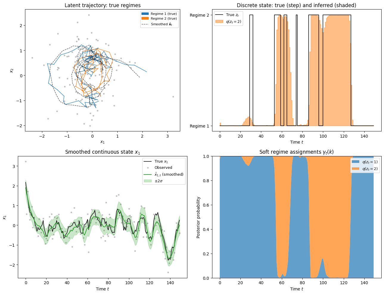

Conclusion¶

The SLDS extends both HMMs and LDS by combining a discrete regime variable with a continuous latent state, enabling models that switch sharply between linear dynamical regimes. The table below places it in context alongside its relatives.

Model	Latent state	Inference algorithm
HMM	$z_t \in \{1,\ldots,K\}$ discrete	Forward-backward
LDS	$\mbx_t \in \reals^{D_x}$ continuous	Kalman filter + RTS smoother
SLDS	$z_t$ discrete $+$ $\mbx_t$ continuous	See below
rSLDS	$z_t$ discrete $+$ $\mbx_t$ continuous, recurrent transitions	See below

The SLDS and rSLDS are hybrid models whose exact posterior is intractable. The table below summarises the main approximation strategies, differing in whether they target the filtered or smoothed posterior and how they represent the continuous state.

Approach	Setting	$q(\mbx_{1:T})$	Handles rSLDS?	Cost per step
Exact (intractable)	Online/offline	$K^t$ Gaussians at step $t$	—	$O(K^T D_x^3)$
Gaussian Sum Filter ( $M$ comp.)	Online	$M$ Gaussians per state	No	$O(M K^2 D_x^3)$
Single-component GSF ( $M=1$ )	Online	1 Gaussian per state	No	$O(K^2 D_x^3)$
Structured mean-field VI	Offline	LDS-chain smoother	Approximately	$O(K D_x^3)$
Variational Laplace EM	Offline	MAP + block-tridiag Hessian	Yes	$O(D_x^3)$ per Newton step