Dirichlet Process Mixture Models

Finite Bayesian mixture models require specifying the number of components $K$ in advance. Dirichlet process mixture models (DPMMs) are a Bayesian nonparametric alternative that allows the number of clusters to grow with the data. In this chapter we derive DPMMs from finite mixture models by taking $K \to \infty$ , then study the random measure perspective and its connection to Poisson processes.

Finite Bayesian Mixture Models¶

A finite Bayesian mixture model with $K$ components is defined by the following generative process:

Sample mixing proportions from a Dirichlet prior with concentration $\boldsymbol{\alpha} \in \mathbb{R}_+^K$ :

\boldsymbol{\pi} \sim \mathrm{Dirichlet}(\boldsymbol{\alpha}).

(1)

Sample component parameters:

\boldsymbol{\theta}_k \overset{\text{iid}}{\sim} p(\boldsymbol{\theta} \mid \boldsymbol{\phi}, \nu) \qquad k = 1, \ldots, K.

(2)

Sample assignments and observations:

z_n \overset{\text{iid}}{\sim} \boldsymbol{\pi}, \qquad \mathbf{x}_n \sim p(\mathbf{x} \mid \boldsymbol{\theta}_{z_n}) \qquad n = 1, \ldots, N.

(3)

The joint distribution factorizes as:

p(\boldsymbol{\pi}, \{\boldsymbol{\theta}_k\}, \{z_n, \mathbf{x}_n\}) = \mathrm{Dir}(\boldsymbol{\pi} \mid \boldsymbol{\alpha}) \prod_{k=1}^K p(\boldsymbol{\theta}_k \mid \boldsymbol{\phi}, \nu) \prod_{n=1}^N \prod_{k=1}^K \left[\pi_k \, p(\mathbf{x}_n \mid \boldsymbol{\theta}_k)\right]^{\mathbb{I}[z_n = k]}.

(4)

Collapsing Out Parameters¶

When the likelihood is an exponential family and the prior is its conjugate,

p(\mathbf{x} \mid \boldsymbol{\theta}_k) = h(\mathbf{x}) \exp\{\langle t(\mathbf{x}), \boldsymbol{\theta}_k \rangle - A(\boldsymbol{\theta}_k)\}, \qquad p(\boldsymbol{\theta}_k \mid \boldsymbol{\phi}, \nu) = \frac{1}{Z_\theta(\boldsymbol{\phi}, \nu)} \exp\{\langle \boldsymbol{\phi}, \boldsymbol{\theta}_k \rangle - \nu A(\boldsymbol{\theta}_k)\},

(5)

we can marginalize (or collapse) the component parameters and mixture proportions in closed form.

After integrating out $\{\boldsymbol{\theta}_k\}$ and $\boldsymbol{\pi}$ , the marginal likelihood over assignments $\{z_n\}$ and observations $\{\mathbf{x}_n\}$ is:

p(\{z_n, \mathbf{x}_n\} \mid \boldsymbol{\phi}, \nu, \boldsymbol{\alpha}) = \frac{Z_\pi(\boldsymbol{\alpha}')}{Z_\pi(\boldsymbol{\alpha})} \prod_{k=1}^K \frac{Z_\theta(\boldsymbol{\phi}_k', \nu_k')}{Z_\theta(\boldsymbol{\phi}, \nu)},

(6)

where the updated hyperparameters are:

\boldsymbol{\alpha}' = [\alpha_1 + N_1, \ldots, \alpha_K + N_K], \qquad \boldsymbol{\phi}_k' = \boldsymbol{\phi} + \sum_{n:\, z_n=k} t(\mathbf{x}_n), \qquad \nu_k' = \nu + N_k,

(7)

and $Z_\pi(\boldsymbol{\alpha}) = \prod_k \Gamma(\alpha_k) / \Gamma(\sum_k \alpha_k)$ is the Dirichlet normalizing constant.

This is a general pattern: in conjugate exponential families, marginal likelihoods are ratios of posterior to prior normalizing functions.

Collapsed Gibbs Sampling¶

Working with the collapsed distribution enables efficient collapsed Gibbs sampling. The conditional distribution of $z_n$ , holding all other assignments fixed, simplifies to:

p(z_n = k \mid \mathbf{x}_n, \{z_{n'}\}_{n' \neq n}, \boldsymbol{\phi}, \nu, \boldsymbol{\alpha}) \propto \underbrace{(\alpha_k + N_k^{(\neg n)})}_{\text{cluster size}} \cdot \underbrace{p(\mathbf{x}_n \mid \{\mathbf{x}_{n'} : z_{n'} = k\}, \boldsymbol{\phi}, \nu)}_{\text{posterior predictive}},

(8)

where $N_k^{(\neg n)} = \sum_{n' \neq n} \mathbb{I}[z_{n'} = k]$ is the number of other points in cluster $k$ .

The two factors have intuitive interpretations:

The cluster size term $\alpha_k + N_k^{(\neg n)}$ comes from the Dirichlet–Multinomial conjugacy: larger clusters attract new points.
The posterior predictive term $p(\mathbf{x}_n \mid \ldots)$ measures how well $\mathbf{x}_n$ fits with the other points in cluster $k$ .

The Dirichlet Process Mixture Model¶

Now set $\boldsymbol{\alpha} = \frac{\alpha}{K} \mathbf{1}_K$ and take $K \to \infty$ . In this limit, the collapsed Gibbs update simplifies to:

p(z_n = k \mid \mathbf{x}_n, \{z_{n'}\}_{n' \neq n}) \propto \begin{cases} N_k^{(\neg n)} \cdot p(\mathbf{x}_n \mid \{\mathbf{x}_{n'} : z_{n'} = k\}, \boldsymbol{\phi}, \nu) & \text{if } k \text{ is an existing cluster} \\ \alpha \cdot p(\mathbf{x}_n \mid \boldsymbol{\phi}, \nu) & \text{if } k \text{ is a new cluster.} \end{cases}

(9)

This is the DPMM collapsed Gibbs update. It is nonparametric — $K$ is never fixed, and the number of occupied clusters can grow or shrink at each step:

A cluster is created when a data point is assigned to a new cluster (probability controlled by $\alpha$ ).
A cluster is deleted when its last data point is reassigned elsewhere.

The parameter $\alpha > 0$ is the concentration: larger $\alpha$ creates more clusters.

The Chinese Restaurant Process (CRP)¶

The prior on partitions induced by the DPMM has a beautiful sequential description called the Chinese restaurant process (CRP). Imagine $N$ customers entering a restaurant one at a time:

Customer 1 sits at a new table.
Customer $n$ sits at an existing table $k$ with probability $\frac{|\mathcal{C}_k|}{\alpha + n - 1}$ , or starts a new table with probability $\frac{\alpha}{\alpha + n - 1}$ .

The resulting partition $\mathcal{C} = \{\mathcal{C}_1, \ldots\}$ is the CRP prior on partitions of $[N]$ .

Stick-Breaking Construction¶

The DPMM can also be defined directly via a random measure:

\Theta = \sum_{k=1}^\infty \pi_k \, \delta_{\boldsymbol{\theta}_k}, \qquad \boldsymbol{\theta}_k \overset{\text{iid}}{\sim} G,

(10)

where the weights follow a stick-breaking construction: sample $\ell_k \sim \mathrm{Beta}(1, \alpha)$ and set

\pi_k = \ell_k \prod_{j=1}^{k-1} (1 - \ell_j).

(11)

We write $\Theta \sim \mathrm{DP}(\alpha, G)$ and call $\alpha$ the concentration and $G$ the base measure.

def normal_log_posterior_predictive(x, cluster_points, mu0, kappa0, alpha0, beta0):
    '''Log posterior predictive p(x | cluster_points) under Normal-NormalInverseGamma prior.

    Model: x_n | mu, sigma^2 ~ N(mu, sigma^2)
           mu | sigma^2 ~ N(mu0, sigma^2 / kappa0)
           sigma^2 ~ IG(alpha0, beta0)

    The marginal p(x | data) is a Student-t distribution.

    Args:
        x: new point, shape (D,)
        cluster_points: tensor of shape (N_k, D); empty if prior predictive
        mu0: prior mean, shape (D,)
        kappa0: prior precision scaling (scalar)
        alpha0: prior shape (scalar)
        beta0: prior rate (scalar)
    Returns:
        log predictive density (scalar)
    '''
    D = x.shape[0]
    n = len(cluster_points)
    if n > 0:
        x_bar = cluster_points.mean(0)
        kappa_n = kappa0 + n
        mu_n = (kappa0 * mu0 + n * x_bar) / kappa_n
        alpha_n = alpha0 + n / 2.0
        S = ((cluster_points - x_bar) ** 2).sum(0)  # shape (D,)
        diff = x_bar - mu0
        beta_n = beta0 + 0.5 * S + 0.5 * kappa0 * n / kappa_n * diff ** 2
    else:
        kappa_n, mu_n, alpha_n, beta_n = kappa0, mu0, alpha0, beta0 * torch.ones(D)

    # Marginal is a Student-t: t(2*alpha_n, mu_n, beta_n*(kappa_n+1)/(alpha_n*kappa_n))
    df = 2.0 * alpha_n
    scale2 = beta_n * (kappa_n + 1) / (alpha_n * kappa_n)
    log_p = 0.0
    for d in range(D):
        log_p += float(student_t.logpdf(x[d].item(), df=df, loc=mu_n[d].item(),
                                         scale=scale2[d].item() ** 0.5))
    return log_p


def collapsed_gibbs_dpmm(X, alpha, mu0, kappa0, alpha0, beta0, num_iters=100, seed=0):
    '''Collapsed Gibbs sampler for a DPMM with Normal-NormalInverseGamma components.

    Args:
        X: data, shape (N, D)
        alpha: DP concentration
        mu0, kappa0, alpha0, beta0: NIG prior hyperparameters
        num_iters: number of Gibbs sweeps
        seed: random seed
    Returns:
        z: final cluster assignments, shape (N,)
        K_history: number of clusters at each iteration
    '''
    torch.manual_seed(seed)
    N, D = X.shape
    mu0 = mu0 * torch.ones(D)

    # Initialize: one cluster per data point
    z = torch.arange(N)
    K_history = []

    for it in range(num_iters):
        for n in range(N):
            # Remove n from its current cluster
            z_n = z[n].item()
            z[n] = -1
            mask_n = (z >= 0)
            unique_ks = z[mask_n].unique().tolist()

            # Compute log probabilities for each existing cluster and a new one
            log_probs = []
            labels = []
            for k in unique_ks:
                pts = X[(z == k)]
                N_k = len(pts)
                log_like = normal_log_posterior_predictive(X[n], pts, mu0, kappa0, alpha0, beta0)
                log_probs.append(np.log(N_k) + log_like)
                labels.append(k)

            # New cluster
            log_like_new = normal_log_posterior_predictive(X[n], X[:0], mu0, kappa0, alpha0, beta0)
            log_probs.append(np.log(alpha) + log_like_new)
            labels.append(max(unique_ks + [-1]) + 1 if unique_ks else 0)

            # Sample
            log_probs = np.array(log_probs)
            log_probs -= log_probs.max()
            probs = np.exp(log_probs)
            probs /= probs.sum()
            chosen = np.random.choice(len(labels), p=probs)
            z[n] = labels[chosen]

        # Re-label clusters 0, 1, 2, ...
        unique_labels = z.unique().tolist()
        remap = {old: new for new, old in enumerate(unique_labels)}
        z = torch.tensor([remap[zi.item()] for zi in z])
        K_history.append(len(unique_labels))

    return z, K_history

torch.manual_seed(1)
np.random.seed(1)

# Generate data from 3 Gaussians
true_means = torch.tensor([[-2.0, 0.0], [2.0, 0.0], [0.0, 2.5]])
true_std = 0.6
N_per = 40
X_list = [true_means[k] + true_std * torch.randn(N_per, 2) for k in range(3)]
X = torch.cat(X_list)
N = len(X)

# Prior hyperparameters
mu0 = torch.zeros(2)
kappa0 = 0.5
alpha0 = 2.0
beta0 = 1.0
alpha_dp = 2.0

z_final, K_hist = collapsed_gibbs_dpmm(X, alpha=alpha_dp, mu0=mu0, kappa0=kappa0,
                                        alpha0=alpha0, beta0=beta0,
                                        num_iters=80, seed=42)

fig, axes = plt.subplots(1, 2, figsize=(11, 4))

# Left: final clustering
K_final = z_final.max().item() + 1
colors = plt.cm.tab10(np.linspace(0, 1, max(K_final, 10)))
for k in range(K_final):
    mask = (z_final == k).numpy()
    axes[0].scatter(X[mask, 0], X[mask, 1], c=[colors[k]], s=20, alpha=0.8)
for km, mu in enumerate(true_means):
    axes[0].scatter(*mu, marker='*', s=200, c='k', zorder=5)
axes[0].set_title(f'DPMM clustering ($\\alpha={alpha_dp}$): {K_final} clusters found')
axes[0].set_xlabel('$x_1$'); axes[0].set_ylabel('$x_2$')

# Right: K over iterations
axes[1].plot(K_hist, color='tab:blue')
axes[1].axhline(3, ls='--', color='k', label='True K=3')
axes[1].set_xlabel('Gibbs iteration')
axes[1].set_ylabel('Number of clusters')
axes[1].set_title('Cluster count over iterations')
axes[1].legend()

plt.tight_layout()
plt.savefig('dpmm_demo.png', dpi=100, bbox_inches='tight')
plt.show()
print(f"Final number of clusters: {K_final}")

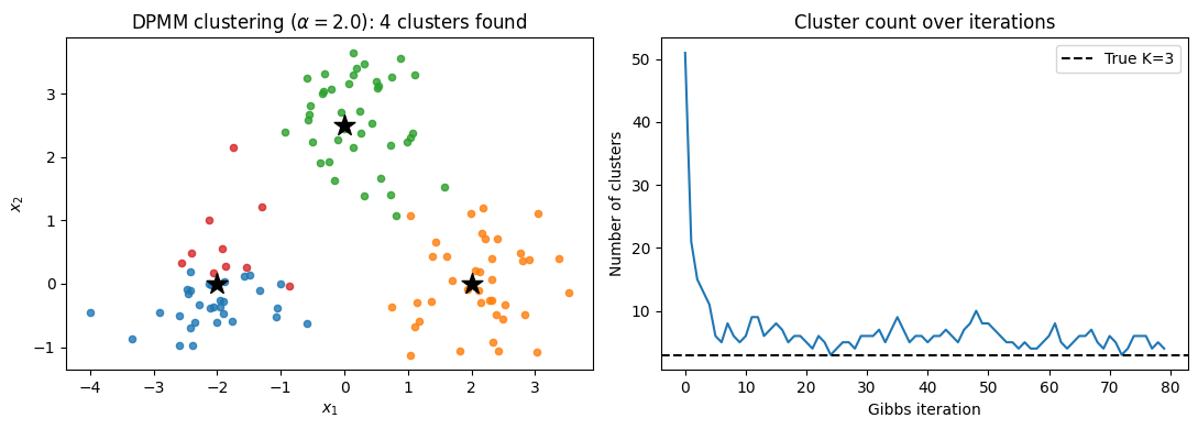
Final number of clusters: 4

Pitman–Yor Process¶

The Pitman–Yor process Orbanz, 2014 generalizes the DP by adding a discount parameter $d \in [0, 1)$ . We write $\Theta \sim \mathrm{PYP}(\alpha, d, G)$ where the weights use the modified stick-breaking:

\ell_k \sim \mathrm{Beta}(1 - d, \, \alpha + kd), \qquad \pi_k = \ell_k \prod_{j=1}^{k-1}(1 - \ell_j).

(12)

When $d = 0$ we recover the DP. When $d > 0$ , the cluster sizes follow a power law, making the PYP well-suited to linguistic data where word frequencies exhibit Zipfian behavior.

The CRP analogue assigns customer $n$ to existing table $k$ with probability $\frac{|\mathcal{C}_k| - d}{\alpha + n - 1}$ or to a new table with probability $\frac{\alpha + d \cdot K^{(n)}}{\alpha + n - 1}$ , where $K^{(n)}$ is the current number of tables.

Mixture of Finite Mixtures¶

DPMMs are often used to select $K$ automatically, but the DP almost surely generates infinitely many clusters as $N \to \infty$ . When the true number of clusters is finite but unknown, mixture of finite mixture models (MFMMs) Miller & Harrison, 2018 are more appropriate:

K \sim p(K), \quad \boldsymbol{\pi} \sim \mathrm{Dir}(\alpha \mathbf{1}_K), \quad \boldsymbol{\theta}_k \overset{\text{iid}}{\sim} G, \quad z_n \overset{\text{iid}}{\sim} \boldsymbol{\pi}, \quad \mathbf{x}_n \sim p(\mathbf{x} \mid \boldsymbol{\theta}_{z_n}).

(13)

A natural choice is $K - 1 \sim \mathrm{Poisson}(\lambda)$ . Collapsed Gibbs samplers for MFMMs have a similar form to the DPMM sampler but converge to a finite $K$ .

Poisson Random Measures¶

Dirichlet processes and Poisson processes are deeply connected. In fact, DPs are instances of completely random measures (CRMs) constructed from Poisson processes.

Random Measures¶

A random measure on $\mathbb{R}^D$ is a measure-valued random variable. An atomic random measure takes the form:

\mu = \sum_{k=1}^\infty w_k \, \delta_{\boldsymbol{\theta}_k},

(14)

where the weights $w_k \in \mathbb{R}_+$ and locations $\boldsymbol{\theta}_k \in \mathbb{R}^D$ are random.

Poisson Random Measures¶

Construct a random measure by sampling weight–location pairs from a marked Poisson process on $\mathbb{R}_+ \times \mathbb{R}^D$ :

\{(w_k, \boldsymbol{\theta}_k)\}_{k=1}^\infty \sim \mathrm{PP}(\lambda(w, \boldsymbol{\theta})).

(15)

For a homogeneous measure the intensity factors: $\lambda(w, \boldsymbol{\theta}) = \lambda(w) \cdot g(\boldsymbol{\theta})$ , where $g$ is a density on $\mathbb{R}^D$ (the base measure $G$ ).

The Gamma Process and Dirichlet Process¶

Choose the weight intensity

\lambda(w) = \alpha w^{-1} e^{-\beta w}.

(16)

Then $\int_0^\infty \lambda(w)\, dw = \infty$ , so $\mu$ has infinitely many atoms. Nevertheless, the total mass $W = \sum_k w_k \sim \mathrm{Gamma}(\alpha, 1/\beta)$ is almost surely finite. This is the gamma process $\mu \sim \mathrm{GaP}(\alpha, G)$ .

Normalizing gives the Dirichlet process:

\mu \sim \mathrm{GaP}(\alpha, G) \quad \Longrightarrow \quad \Theta = \frac{\mu}{W} = \sum_{k=1}^\infty \frac{w_k}{W} \, \delta_{\boldsymbol{\theta}_k} \sim \mathrm{DP}(\alpha, G).

(17)

This is a key result: Dirichlet processes are normalized gamma processes.

Other Completely Random Measures¶

Different weight intensities yield other useful random measures:

Weight intensity $\lambda(w)$	Name
$\alpha w^{-1} e^{-\beta w}$	Gamma process → DP (after normalization)
$\gamma w^{-(\alpha+1)}$	Stable process
$\gamma w^{-1}(1-w)^{\alpha-1}$	Beta process

A CRM $\mu$ has the remarkable property that $\Theta = \mu/W$ is independent of $W$ if and only if $\mu$ is a gamma process — the DP is the unique normalized CRM with this independence property Orbanz, 2014.

Dirichlet Process Mixture Models

Finite Bayesian Mixture Models¶

Collapsing Out Parameters¶

Collapsed Gibbs Sampling¶

The Dirichlet Process Mixture Model¶

The Chinese Restaurant Process (CRP)¶

Stick-Breaking Construction¶

Extensions and Related Models¶

Pitman–Yor Process¶

Mixture of Finite Mixtures¶

Poisson Random Measures¶

Random Measures¶

Poisson Random Measures¶

The Gamma Process and Dirichlet Process¶

Other Completely Random Measures¶