Gaussian Processes

A Gaussian process (GP) is a distribution over functions. Rather than placing a prior over a finite set of parameters, a GP places a prior over the function itself, giving a flexible non-parametric approach to regression and classification. This chapter covers:

The GP definition and common kernels
Exact GP regression
GP classification via augmentation
Elliptical slice sampling
Sparse GPs and inducing points

<torch._C.Generator at 0x7f9514bcb9f0>

Gaussian Processes¶

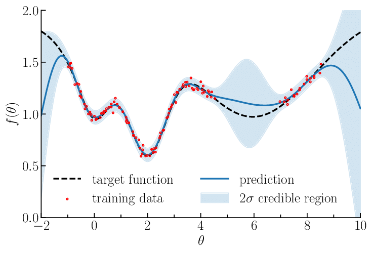
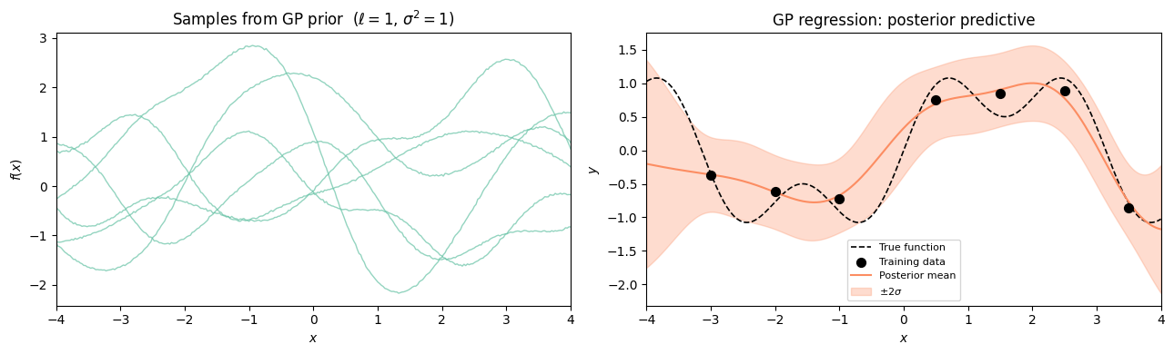
A Gaussian process prior (shaded) and posterior (narrower shaded region)
after conditioning on a few observations (dots). — A Gaussian process prior (shaded) and posterior (narrower shaded region) after conditioning on a few observations (dots).

We say $f \sim \mathcal{GP}(\mu(\cdot), K(\cdot, \cdot))$ if for every finite set of inputs $\{\mathbf{x}_1, \ldots, \mathbf{x}_N\} \subset \mathbb{R}^D$ , the joint distribution of the function values is Gaussian:

\begin{bmatrix} f(\mathbf{x}_1) \\ \vdots \\ f(\mathbf{x}_N) \end{bmatrix} \sim \mathcal{N}\!\left( \begin{bmatrix} \mu(\mathbf{x}_1) \\ \vdots \\ \mu(\mathbf{x}_N) \end{bmatrix},\; \begin{bmatrix} K(\mathbf{x}_1, \mathbf{x}_1) & \cdots & K(\mathbf{x}_1, \mathbf{x}_N) \\ \vdots & & \vdots \\ K(\mathbf{x}_N, \mathbf{x}_1) & \cdots & K(\mathbf{x}_N, \mathbf{x}_N) \end{bmatrix} \right).

(1)

Here $\mu: \mathbb{R}^D \to \mathbb{R}$ is the mean function and $K: \mathbb{R}^D \times \mathbb{R}^D \to \mathbb{R}$ is the kernel (covariance function). The matrix of kernel evaluations is called the Gram matrix. The kernel must be positive definite: the Gram matrix must be PD for every finite set of inputs.

From Linear Regression to GPs¶

GPs are the natural limit of Bayesian linear regression with infinitely many features. Recall that with feature map $\boldsymbol{\phi}(x) = (\phi_1(x), \ldots, \phi_P(x))^\top$ and Gaussian prior $\mathbf{w} \sim \mathcal{N}(\mathbf{0}, \frac{\lambda}{P}\mathbf{I})$ , the function $f(x) = \boldsymbol{\phi}(x)^\top \mathbf{w}$ is a GP with kernel

K(x_i, x_j) = \frac{\lambda}{P}\, \boldsymbol{\phi}(x_i)^\top \boldsymbol{\phi}(x_j).

(2)

Example: squared exponential kernel. Use radial basis function features $\phi_p(x) = e^{-(x - c_p)^2 / 2\ell^2}$ centred at $P$ equally-spaced points. Taking $P \to \infty$ :

\lim_{P\to\infty} K(x_i, x_j) = \lambda \int_{-\infty}^\infty e^{-(x_i-c)^2/2\ell^2} e^{-(x_j-c)^2/2\ell^2}\,dc = \sqrt{\pi}\ell\lambda\; e^{-(x_i-x_j)^2/4\ell^2}.

(3)

This is the squared exponential (SE) kernel (also called the RBF or Gaussian kernel):

K_{\mathrm{SE}}(x_i, x_j) = \sigma^2 \exp\!\left(-\frac{(x_i-x_j)^2}{2\ell^2}\right).

(4)

The SE kernel corresponds to functions that are infinitely differentiable. The length-scale $\ell$ controls how quickly the function varies; $\sigma^2$ is the marginal variance.

Kernels¶

The Matérn Family¶

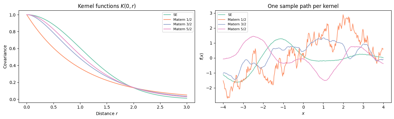
For many applications (e.g. spatial statistics, physical systems), functions are smooth but not infinitely differentiable. The Matérn family provides a spectrum of smoothness controlled by $\nu > 0$ :

K_\nu(x_i, x_j) = \frac{2^{1-\nu}}{\Gamma(\nu)} \left(\frac{\sqrt{2\nu}\,|x_i-x_j|}{\ell}\right)^\nu \mathcal{K}_\nu\!\left(\frac{\sqrt{2\nu}\,|x_i-x_j|}{\ell}\right)

(5)

where $\mathcal{K}_\nu$ is the modified Bessel function. Special cases:

$\nu$	Kernel	GP sample paths
$1/2$	$e^{-\|\Delta\|/\ell}$	Continuous, non-differentiable (OU process)
$3/2$	$(1 + \frac{\sqrt{3}\|\Delta\|}{\ell})e^{-\sqrt{3}\|\Delta\|/\ell}$	Once differentiable
$5/2$	$(1 + \frac{\sqrt{5}\|\Delta\|}{\ell} + \frac{5\|\Delta\|^2}{3\ell^2})e^{-\sqrt{5}\|\Delta\|/\ell}$	Twice differentiable
$\infty$	$e^{-\|\Delta\|^2/2\ell^2}$	Infinitely differentiable (SE)

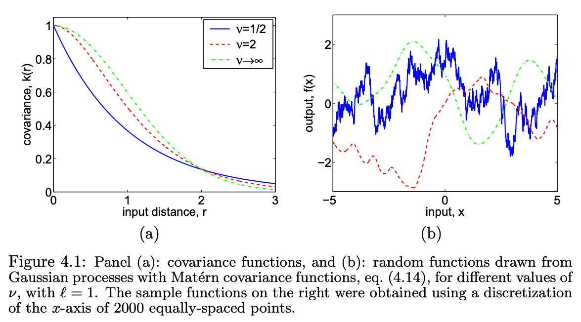
Matérn kernel sample paths for \nu = 1/2, 3/2, 5/2 and the SE (\nu=\infty). — Matérn kernel sample paths for $\nu = 1/2, 3/2, 5/2$ and the SE ( $\nu=\infty$ ).

Stationary Kernels and Bochner’s Theorem¶

Both SE and Matérn kernels are stationary: $K(\mathbf{x}_i, \mathbf{x}_j)$ depends only on the difference $\boldsymbol{\Delta} = \mathbf{x}_i - \mathbf{x}_j$ .

Composing Kernels¶

Kernels can be combined to encode richer structure:

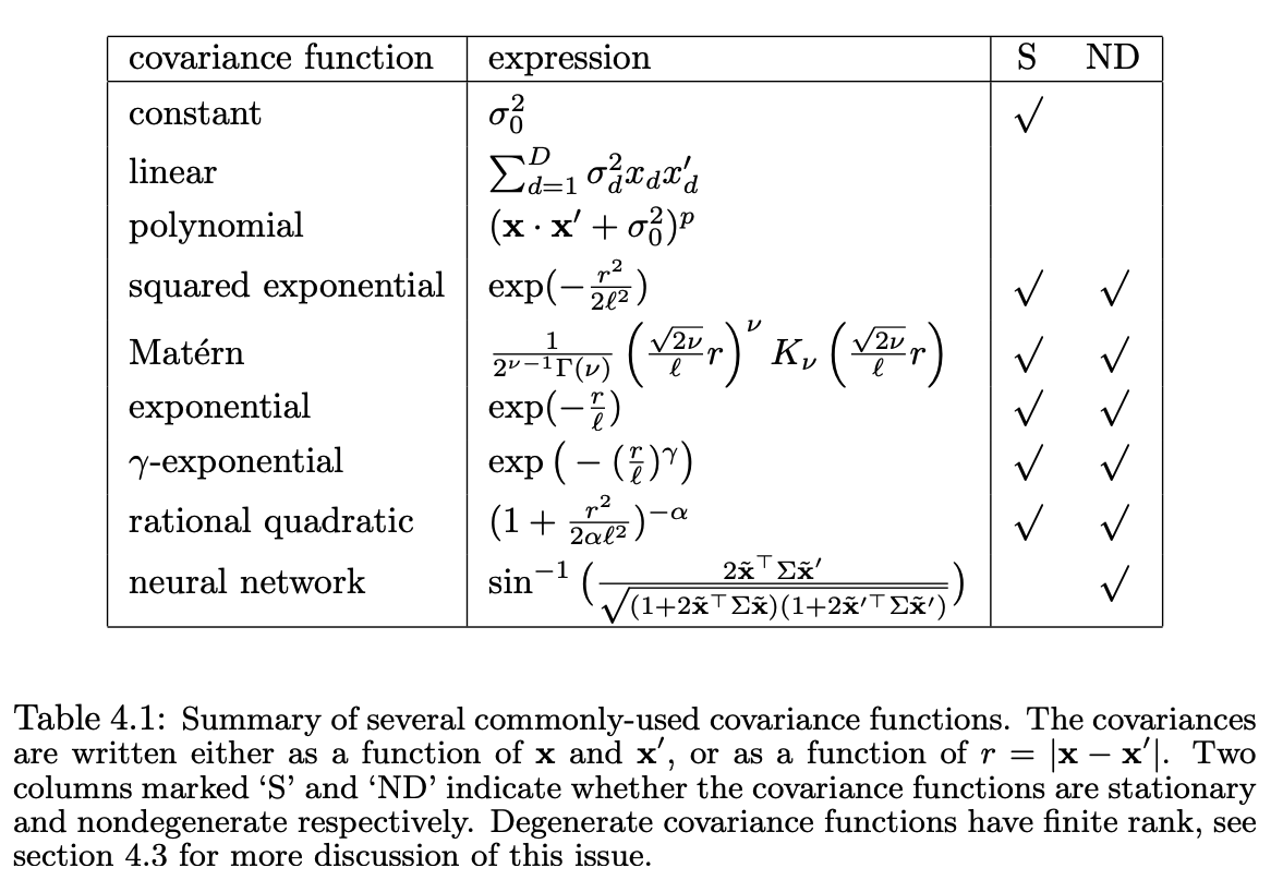
Common kernel functions and their properties.
From . — Common kernel functions and their properties. From Williams & Rasmussen, 1996.

Rules for combining kernels (sums, products, compositions) and what structure
each combination encodes. From the Kernel Cookbook. — Rules for combining kernels (sums, products, compositions) and what structure each combination encodes. From the Kernel Cookbook.

Duvenaud et al., 2013 automated the search over kernel compositions to find the one that best explains a dataset — an approach they called the Automated Statistician.

GP Regression¶

Posterior over Function Values¶

Given observations $(\mathbf{x}_n, y_n)$ with $y_n = f(\mathbf{x}_n) + \epsilon_n$ , $\epsilon_n \sim \mathcal{N}(0, \sigma^2)$ , the posterior over the $N$ -vector $\mathbf{f} = [f(\mathbf{x}_1),\ldots,f(\mathbf{x}_N)]^\top$ is Gaussian:

p(\mathbf{f} \mid \mathbf{y}) = \mathcal{N}(\mathbf{f} \mid \boldsymbol{\mu}', \mathbf{K}')

(7)

\mathbf{K}' = \bigl(\mathbf{K}^{-1} + \sigma^{-2}\mathbf{I}\bigr)^{-1}, \qquad \boldsymbol{\mu}' = \mathbf{K}'\bigl(\mathbf{K}^{-1}\boldsymbol{\mu} + \sigma^{-2}\mathbf{y}\bigr).

(8)

Marginal Likelihood¶

Integrating out $\mathbf{f}$ gives a closed-form marginal likelihood:

p(\mathbf{y}) = \mathcal{N}(\mathbf{y} \mid \boldsymbol{\mu},\, \mathbf{K} + \sigma^2\mathbf{I}).

(9)

This can be used to select hyperparameters (kernel parameters, noise variance) by maximising $\log p(\mathbf{y})$ .

Posterior Predictive Distribution¶

For a new input $\mathbf{x}_\star$ , the joint of $(\mathbf{y}, y_\star)$ is Gaussian. Applying the Schur complement (Chapter 2) yields:

y_\star \mid \mathbf{x}_\star, \mathcal{D} \sim \mathcal{N}(m_\star,\, v_\star)

(10)

m_\star = \mu(\mathbf{x}_\star) + \mathbf{k}_\star^\top(\mathbf{K}+\sigma^2\mathbf{I})^{-1}(\mathbf{y}-\boldsymbol{\mu})

(11)

v_\star = K(\mathbf{x}_\star,\mathbf{x}_\star) + \sigma^2 - \mathbf{k}_\star^\top(\mathbf{K}+\sigma^2\mathbf{I})^{-1}\mathbf{k}_\star

(12)

where $\mathbf{k}_\star = [K(\mathbf{x}_1,\mathbf{x}_\star),\ldots,K(\mathbf{x}_N,\mathbf{x}_\star)]^\top$ .

Computational cost. Computing $(\mathbf{K}+\sigma^2\mathbf{I})^{-1}$ via Cholesky takes $O(N^3)$ time and $O(N^2)$ memory — the key bottleneck for large datasets. The predictive mean has the form $m_\star = \sum_n \alpha_n y_n$ , a linear predictor in the training targets.

GP Classification via Augmentation¶

For binary observations $y_n \in \{0, 1\}$ , a natural model is:

f \sim \mathcal{GP}(\mu(\cdot), K(\cdot, \cdot)), \qquad y_n \sim \mathrm{Bernoulli}(g(f(\mathbf{x}_n))),

(13)

where $g$ is the probit or logistic link. The posterior $p(\mathbf{f} \mid \{\mathbf{x}_n, y_n\})$ is no longer Gaussian.

Probit Augmentation¶

Albert & Chib, 1993 and Girolami & Rogers, 2006 exploit the identity

\Phi(f) = \Pr(z \le f) = \int_0^\infty \mathcal{N}(z \mid f, 1)\,dz, \quad z \sim \mathcal{N}(0,1),

(14)

to introduce auxiliary variables $z_n$ :

p(y_n \mid z_n) = \begin{cases} \mathbf{1}[z_n > 0] & y_n = 1 \\ \mathbf{1}[z_n \le 0] & y_n = 0 \end{cases} \qquad z_n \mid f(\mathbf{x}_n) \sim \mathcal{N}(f(\mathbf{x}_n), 1).

(15)

The augmented posterior factorises cleanly, enabling a Gibbs sampler:

p(\mathbf{f}, \{z_n\} \mid \{\mathbf{x}_n, y_n\}) \propto \prod_n p(y_n \mid z_n)\,\mathcal{N}(z_n \mid f(\mathbf{x}_n), 1)\cdot\mathcal{N}(\mathbf{f} \mid \boldsymbol{\mu}, \mathbf{K}).

(16)

Conditional updates:

$z_n \mid \mathbf{f}, y_n$ : truncated Gaussian — $\mathcal{N}(f(\mathbf{x}_n), 1)$ truncated to $(0, \infty)$ if $y_n=1$ , to $(-\infty, 0]$ if $y_n=0$ .
$\mathbf{f} \mid \{z_n\}$ : standard GP regression with Gaussian observations $z_n \sim \mathcal{N}(f(\mathbf{x}_n), 1)$ .

Elliptical Slice Sampling¶

For non-conjugate GP models (e.g. GP classification with a logistic link), standard Gibbs can mix poorly because the GP prior induces strong correlations between function values.

Murray et al., 2010 proposed elliptical slice sampling (ESS), which exploits the Gaussian structure of the prior. The key observation is that any draw from $\mathcal{N}(\mathbf{0}, \boldsymbol{\Sigma})$ can be written as

\mathbf{f} = \boldsymbol{\nu}_0 \sin\theta + \boldsymbol{\nu}_1 \cos\theta, \qquad \boldsymbol{\nu}_0, \boldsymbol{\nu}_1 \sim \mathcal{N}(\mathbf{0}, \boldsymbol{\Sigma}).

(17)

Given the current $\mathbf{f}$ , a new proposal is made by rotating on the ellipse defined by $\mathbf{f}$ and a fresh auxiliary draw $\boldsymbol{\nu}$ :

\mathbf{f}' = \mathbf{f}\cos\theta + \boldsymbol{\nu}\sin\theta, \qquad \boldsymbol{\nu} \sim \mathcal{N}(\mathbf{0}, \boldsymbol{\Sigma}).

(18)

The angle $\theta$ is sampled by a slice over $[0, 2\pi)$ : start with a random bracket, evaluate the likelihood at the proposal, shrink the bracket if the proposal is rejected. The algorithm is always accepted eventually and leaves the posterior invariant.

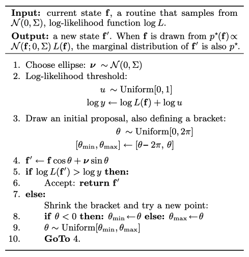
ESS proposes moves along an ellipse in function space, automatically
respecting the GP prior covariance structure. — ESS proposes moves along an ellipse in function space, automatically respecting the GP prior covariance structure.

Sparse GPs and Inducing Points¶

Exact GP inference costs $O(N^3)$ . For large $N$ we need approximations. Inducing point methods Titsias, 2009 introduce $M \ll N$ pseudo-inputs $\{\mathbf{z}_m\}$ and approximate the full posterior with one conditioned on the function values $\mathbf{u} = [f(\mathbf{z}_1),\ldots,f(\mathbf{z}_M)]^\top$ .

Using the GP predictive distribution:

p(\mathbf{f} \mid \mathbf{u}) = \mathcal{N}(\mathbf{f} \mid \mathbf{K}_{NM}\mathbf{K}_{MM}^{-1}\mathbf{u},\; \tilde{\mathbf{K}}) \qquad \tilde{\mathbf{K}} = \mathbf{K}_{NN} - \mathbf{K}_{NM}\mathbf{K}_{MM}^{-1}\mathbf{K}_{MN}.

(19)

Variational Bound¶

Titsias, 2009 lower-bounds $\log p(\mathbf{y})$ by:

\mathcal{L}_2 = \log \mathcal{N}(\mathbf{y} \mid \mathbf{0},\; \mathbf{K}_{NM}\mathbf{K}_{MM}^{-1}\mathbf{K}_{MN} + \sigma^2\mathbf{I}) - \frac{1}{2\sigma^2}\mathrm{tr}(\tilde{\mathbf{K}}).

(20)

The first term is the likelihood of a low-rank GP; the trace term penalises unexplained prior variance. Computing $\mathcal{L}_2$ costs $O(NM^2 + M^3)$ .

Stochastic Variational Inference¶

Hensman et al., 2013 showed that if we explicitly maintain a variational distribution $q(\mathbf{u}) = \mathcal{N}(\mathbf{m}, \mathbf{S})$ rather than marginalising out $\mathbf{u}$ , the ELBO factorises over data points:

\mathcal{L}_3 = \sum_{n=1}^N \mathbb{E}_{q(f(\mathbf{x}_n))}[\log p(y_n \mid f(\mathbf{x}_n))] - \mathrm{KL}(q(\mathbf{u}) \| p(\mathbf{u})).

(21)

This enables mini-batch stochastic gradient ascent, scaling GPs to millions of observations at $O(M^3)$ per step.

# ── Kernel functions ──────────────────────────────────────────────────────────

def rbf_kernel(x1, x2, length_scale=1.0, variance=1.0):
    '''Squared exponential (RBF) kernel  k(x1, x2) = variance * exp(-r^2 / 2).

    Args:
        x1: (N1,)  1-D inputs
        x2: (N2,)  1-D inputs
    Returns:
        (N1, N2) Gram matrix
    '''
    r2 = ((x1[:, None] - x2[None, :]) / length_scale) ** 2
    return variance * torch.exp(-0.5 * r2)


def matern_kernel(x1, x2, length_scale=1.0, variance=1.0, nu=1.5):
    '''Matern kernel for nu in {0.5, 1.5, 2.5}.

    Args:
        x1: (N1,)  1-D inputs
        x2: (N2,)  1-D inputs
        nu: smoothness parameter (0.5, 1.5, or 2.5)
    Returns:
        (N1, N2) Gram matrix
    '''
    r = (x1[:, None] - x2[None, :]).abs() / length_scale
    if nu == 0.5:
        return variance * torch.exp(-r)
    elif nu == 1.5:
        sr = math.sqrt(3) * r
        return variance * (1 + sr) * torch.exp(-sr)
    elif nu == 2.5:
        sr = math.sqrt(5) * r
        return variance * (1 + sr + sr**2 / 3) * torch.exp(-sr)
    else:
        raise ValueError(f'Unsupported nu={nu}; use 0.5, 1.5, or 2.5')


# ── Exact GP regression ───────────────────────────────────────────────────────

def gp_posterior_predictive(x_train, y_train, x_test, kernel_fn,
                             noise_var=0.1, mu=0.0):
    '''Exact GP regression: posterior predictive mean and std.

    Model:
        f ~ GP(mu, K)
        y_n | f ~ N(f(x_n), noise_var)

    Args:
        x_train:    (N,)   training inputs
        y_train:    (N,)   training targets
        x_test:     (M,)   test inputs
        kernel_fn:  callable(x1, x2) -> (N1, N2) kernel matrix
        noise_var:  observation noise variance
        mu:         prior mean (scalar)
    Returns:
        mean_pred:  (M,)   posterior predictive mean
        std_pred:   (M,)   posterior predictive std
        log_ml:     scalar log marginal likelihood
    '''
    N = len(x_train)
    jitter = 1e-4

    K_nn = kernel_fn(x_train, x_train) + (noise_var + jitter) * torch.eye(N)  # jitter=1e-4
    k_ns = kernel_fn(x_train, x_test)   # (N, M)
    K_ss = kernel_fn(x_test,  x_test)   # (M, M)

    L     = torch.linalg.cholesky(K_nn)                        # (N, N)
    alpha = torch.cholesky_solve((y_train - mu).unsqueeze(1), L).squeeze(1)  # (N,)

    mean_pred = mu + k_ns.T @ alpha                             # (M,)

    v         = torch.linalg.solve_triangular(L, k_ns, upper=False)  # (N, M)
    var_pred   = K_ss.diagonal() - (v * v).sum(0)              # (M,)
    var_pred   = var_pred.clamp(min=0) + noise_var
    std_pred   = var_pred.sqrt()

    # Log marginal likelihood: log N(y | mu*1, K_nn)
    log_ml = (-0.5 * (y_train - mu) @ alpha
              - L.diagonal().log().sum()
              - 0.5 * N * math.log(2 * math.pi))

    return mean_pred, std_pred, log_ml

import numpy as np

# ── Helper: sample prior paths ────────────────────────────────────────────────
def sample_prior(x, kernel_fn, n_samples=5, seed=0):
    torch.manual_seed(seed)
    K = kernel_fn(x, x) + 1e-4 * torch.eye(len(x))
    L = torch.linalg.cholesky(K)
    eps = torch.randn(len(x), n_samples)
    return L @ eps   # (N, n_samples)

# ── GP regression demo ────────────────────────────────────────────────────────
x_all  = torch.linspace(-4, 4, 300)

# True function
f_true = lambda x: torch.sin(x) + 0.5 * torch.sin(3 * x)

# Training data
torch.manual_seed(7)
x_train = torch.tensor([-3.0, -2.0, -1.0, 0.5, 1.5, 2.5, 3.5])
y_train = f_true(x_train) + 0.2 * torch.randn(len(x_train))

# Kernel choice
ell, sigma2 = 1.0, 1.0
kfn = lambda a, b: rbf_kernel(a, b, length_scale=ell, variance=sigma2)

mean_pred, std_pred, log_ml = gp_posterior_predictive(
    x_train, y_train, x_all, kfn, noise_var=0.04)

print(f'Log marginal likelihood: {log_ml:.2f}')

# ── Plot ──────────────────────────────────────────────────────────────────────
fig, axes = plt.subplots(1, 2, figsize=(13, 4))

# Panel 1: prior samples
ax = axes[0]
prior_samples = sample_prior(x_all, kfn, n_samples=6)
for i in range(prior_samples.shape[1]):
    ax.plot(x_all.numpy(), prior_samples[:, i].numpy(),
            lw=1.0, alpha=0.7, color=palette[0])
ax.set_title('Samples from GP prior  ($\ell=1$, $\sigma^2=1$)')
ax.set_xlabel('$x$')
ax.set_ylabel('$f(x)$')
ax.set_xlim(-4, 4)

# Panel 2: posterior predictive
ax = axes[1]
mu_np  = mean_pred.numpy()
std_np = std_pred.numpy()
x_np   = x_all.numpy()

ax.plot(x_np, f_true(x_all).numpy(), 'k--', lw=1.2, label='True function')
ax.scatter(x_train.numpy(), y_train.numpy(), s=50, zorder=5,
           color='k', label='Training data')
ax.plot(x_np, mu_np, color=palette[1], lw=1.5, label='Posterior mean')
ax.fill_between(x_np, mu_np - 2*std_np, mu_np + 2*std_np,
                alpha=0.3, color=palette[1], label='$\pm 2\sigma$')
ax.set_title('GP regression: posterior predictive')
ax.set_xlabel('$x$')
ax.set_ylabel('$y$')
ax.set_xlim(-4, 4)
ax.legend(fontsize=8)

plt.tight_layout()
plt.show()

# ── Kernel comparison plot ────────────────────────────────────────────────────
fig, axes = plt.subplots(1, 2, figsize=(13, 4))

kernels = [
    ('SE', lambda a, b: rbf_kernel(a, b, length_scale=1.0)),
    ('Matern 1/2', lambda a, b: matern_kernel(a, b, length_scale=1.0, nu=0.5)),
    ('Matern 3/2', lambda a, b: matern_kernel(a, b, length_scale=1.0, nu=1.5)),
    ('Matern 5/2', lambda a, b: matern_kernel(a, b, length_scale=1.0, nu=2.5)),
]
x_dense = torch.linspace(-4, 4, 300)

# Kernel values vs distance
ax = axes[0]
dists = torch.linspace(0, 3, 200)
x0    = torch.zeros(1)
for i, (name, kfn_i) in enumerate(kernels):
    k_vals = kfn_i(x0, dists).squeeze()
    ax.plot(dists.numpy(), k_vals.detach().numpy(), label=name,
            lw=1.5, color=palette[i])
ax.set_title('Kernel functions $K(0, r)$')
ax.set_xlabel('Distance $r$')
ax.set_ylabel('Covariance')
ax.legend(fontsize=8)

# Sample paths per kernel
ax = axes[1]
for i, (name, kfn_i) in enumerate(kernels):
    s = sample_prior(x_dense, kfn_i, n_samples=1, seed=i)
    ax.plot(x_dense.numpy(), s[:, 0].detach().numpy(),
            label=name, lw=1.3, color=palette[i])
ax.set_title('One sample path per kernel')
ax.set_xlabel('$x$')
ax.set_ylabel('$f(x)$')
ax.legend(fontsize=8)

plt.tight_layout()
plt.show()

<>:40: SyntaxWarning: invalid escape sequence '\e'
<>:56: SyntaxWarning: invalid escape sequence '\p'
<>:40: SyntaxWarning: invalid escape sequence '\e'
<>:56: SyntaxWarning: invalid escape sequence '\p'
/tmp/ipykernel_2781/395890649.py:40: SyntaxWarning: invalid escape sequence '\e'
  ax.set_title('Samples from GP prior  ($\ell=1$, $\sigma^2=1$)')
/tmp/ipykernel_2781/395890649.py:56: SyntaxWarning: invalid escape sequence '\p'
  alpha=0.3, color=palette[1], label='$\pm 2\sigma$')

Log marginal likelihood: -7.93

Conclusion¶

Topic	Key result
GP prior	Any finite marginal is Gaussian; kernel encodes structure
SE kernel	Limit of linear regression with infinitely many RBF features
GP regression	Posterior and predictive in closed form via Schur complement
Marginal likelihood	$\mathcal{N}(\mathbf{y}\mid\boldsymbol{\mu}, \mathbf{K}+\sigma^2\mathbf{I})$ ; used to tune hyperparameters
GP classification	Probit augmentation converts to Gaussian observations
Elliptical slice sampling	Slice sampling respecting GP prior correlations
Sparse GPs	$O(NM^2)$ inference; SVI enables mini-batch training

Key limitation. Exact GP inference costs $O(N^3)$ . Sparse / inducing point methods reduce this, but designing scalable, expressive GP models remains an active research area.

References¶

Williams, C. K., & Rasmussen, C. E. (1996). Gaussian processes for regression. MIT Press.
Duvenaud, D., Lloyd, J., Grosse, R., Tenenbaum, J., & Zoubin, G. (2013). Structure discovery in nonparametric regression through compositional kernel search. International Conference on Machine Learning, 1166–1174.
Albert, J. H., & Chib, S. (1993). Bayesian analysis of binary and polychotomous response data. Journal of the American Statistical Association, 88(422), 669–679.
Girolami, M., & Rogers, S. (2006). Variational Bayesian multinomial probit regression with Gaussian process priors. Neural Computation, 18(8), 1790–1817.
Murray, I., Adams, R., & MacKay, D. (2010). Elliptical slice sampling. Proceedings of the Thirteenth International Conference on Artificial Intelligence and Statistics, 541–548.
Titsias, M. (2009). Variational Learning of Inducing Variables in Sparse Gaussian Processes. In D. van Dyk & M. Welling (Eds.), Proceedings of the Twelth International Conference on Artificial Intelligence and Statistics (Vol. 5, pp. 567–574). PMLR.
Hensman, J., Fusi, N., & Lawrence, N. D. (2013). Gaussian processes for Big data. Proceedings of the Twenty-Ninth Conference on Uncertainty in Artificial Intelligence, 282–290.