Poisson Processes

Poisson processes are fundamental stochastic models for random sets of points in time or space. In this chapter we study their defining properties, four ways to sample them, and how to go beyond simple Poisson models with self-exciting and doubly stochastic processes.

Defining Properties of a Poisson Process¶

A Poisson process is a stochastic process that generates a random set of points $\{\mathbf{x}_n\}_{n=1}^N \subset \mathcal{X}$ . It is governed by an intensity function $\lambda(\mathbf{x}): \mathcal{X} \to \mathbb{R}_+$ .

Two key properties define a Poisson process:

Property 1 (Poisson counts): The number of points in any measurable set $\mathcal{A}$ follows a Poisson distribution,
$N(\mathcal{A}) \sim \mathrm{Poisson}\!\left(\int_{\mathcal{A}} \lambda(\mathbf{x})\, d\mathbf{x} \right).$
(1)
Property 2 (Independence): Counts on disjoint sets are independent,
$N(\mathcal{A}) \perp N(\mathcal{B}) \iff \mathcal{A} \cap \mathcal{B} = \varnothing.$
(2)

An inhomogeneous Poisson process on [0, T] with a time-varying intensity \lambda(t). — An inhomogeneous Poisson process on $[0, T]$ with a time-varying intensity $\lambda(t)$ .

Common applications include modeling neural spike trains, locations of trees in a forest, arrival times of customers or web requests, and positions of photons on a detector.

Poisson Process Likelihood¶

From the top-down sampling procedure we can derive the likelihood. Given points $\{x_n\}_{n=1}^N \subset [0, T]$ :

p\!\left(\{x_n\}_{n=1}^N \mid \lambda\right) = e^{-\int_0^T \lambda(x)\, dx} \prod_{n=1}^N \lambda(x_n).

(3)

This can be understood as: the probability that no point falls outside the observed set (the exponential factor) times the probability density at each observed location (the product term).

Four Ways to Sample a Poisson Process¶

1. Top-Down Sampling¶

For a Poisson process with intensity $\lambda(\mathbf{x})$ on domain $\mathcal{X}$ :

Sample the total count $N \sim \mathrm{Poisson}\!\left(\int_{\mathcal{X}} \lambda(\mathbf{x})\, d\mathbf{x}\right)$ .
Sample locations i.i.d. from the normalized intensity,
$\mathbf{x}_n \overset{\text{iid}}{\sim} \frac{\lambda(\mathbf{x})}{\int_{\mathcal{X}} \lambda(\mathbf{x}')\, d\mathbf{x}'}.$
(4)

This requires the ability to compute the integral of $\lambda$ and to sample from the normalized intensity.

2. Interval Sampling (Homogeneous Case)¶

A homogeneous Poisson process has constant intensity $\lambda(\mathbf{x}) \equiv \lambda$ .

Property 3: Inter-arrival times are i.i.d. exponential,

\Delta_n = x_n - x_{n-1} \overset{\text{iid}}{\sim} \mathrm{Exp}(\lambda).

(5)

Property 4 (Memoryless): The waiting time until the next point is independent of time elapsed since the last point.

Algorithm: start at $x_0 = 0$ , repeatedly sample $\Delta_n \sim \mathrm{Exp}(\lambda)$ and set $x_n = x_{n-1} + \Delta_n$ , stopping when $x_n > T$ .

3. Time-Rescaling (Inhomogeneous Case)¶

Define the cumulative intensity $\Lambda(x) = \int_0^x \lambda(t)\, dt$ . When $\lambda > 0$ everywhere, $\Lambda$ is invertible.

Algorithm:

Sample a homogeneous Poisson process with unit rate on $[0, \Lambda(T)]$ to get $\mathbf{U} = \{u_n\}$ .
Set $\mathbf{X} = \{\Lambda^{-1}(u_n) : u_n \in \mathbf{U}\}$ .

This is the point-process analog of inverse-CDF sampling.

4. Thinning (Rejection Sampling)¶

Given a bounded intensity $\lambda(\mathbf{x}) \leq \lambda_{\max}$ :

Sample a homogeneous Poisson process with rate $\lambda_{\max}$ to get candidate points.
Independently accept each candidate $\mathbf{x}$ with probability $\lambda(\mathbf{x}) / \lambda_{\max}$ .

This is the point-process analog of rejection sampling.

def sample_pp_topdown(intensity_fn, total_intensity, sample_location_fn, T):
    '''Sample an inhomogeneous Poisson process using the top-down method.

    Args:
        intensity_fn: callable, intensity at a point
        total_intensity: integral of intensity over [0, T]
        sample_location_fn: callable returning one sample from normalized intensity
        T: end of interval
    Returns:
        sorted array of event times
    '''
    N = torch.poisson(torch.tensor(total_intensity)).int().item()
    events = torch.tensor([sample_location_fn() for _ in range(N)])
    return events.sort().values


def sample_pp_intervals(lam, T):
    '''Sample a homogeneous Poisson process on [0, T] via inter-arrival intervals.

    Args:
        lam: rate (scalar)
        T: end of interval
    Returns:
        1D tensor of event times
    '''
    events = []
    t = 0.0
    while True:
        dt = torch.distributions.Exponential(torch.tensor(lam)).sample().item()
        t += dt
        if t > T:
            break
        events.append(t)
    return torch.tensor(events)


def sample_pp_thinning(intensity_fn, lam_max, T, dt=1e-3):
    '''Sample an inhomogeneous Poisson process on [0, T] via thinning.

    Args:
        intensity_fn: callable mapping time -> intensity (must be <= lam_max)
        lam_max: upper bound on intensity
        T: end of interval
        dt: time resolution (unused here; thinning uses continuous time)
    Returns:
        1D tensor of accepted event times
    '''
    candidates = sample_pp_intervals(lam_max, T)
    accepted = []
    for t in candidates:
        prob = intensity_fn(t.item()) / lam_max
        if torch.rand(1).item() < prob:
            accepted.append(t.item())
    return torch.tensor(accepted)

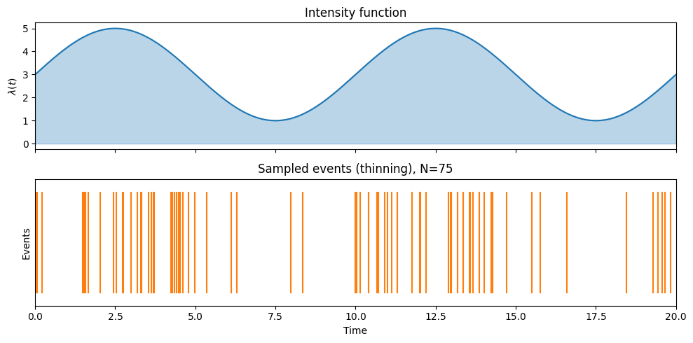
torch.manual_seed(42)
np.random.seed(42)

T = 20.0

# Define a sinusoidal intensity: lambda(t) = 3 + 2*sin(pi*t/5)
def intensity(t):
    return 3.0 + 2.0 * np.sin(np.pi * t / 5.0)

lam_max = 5.0
total_lam = 3.0 * T  # integral of constant part; sin integrates to 0

fig, axes = plt.subplots(2, 1, figsize=(10, 5), sharex=True)

# Plot intensity
ts = np.linspace(0, T, 500)
axes[0].fill_between(ts, intensity(ts), alpha=0.3, color='tab:blue')
axes[0].plot(ts, intensity(ts), color='tab:blue')
axes[0].set_ylabel(r'$\lambda(t)$')
axes[0].set_title('Intensity function')

# Sample via thinning
events_thin = sample_pp_thinning(intensity, lam_max, T)
axes[1].eventplot(events_thin.numpy(), lineoffsets=0.5, linelengths=0.8, color='tab:orange')
axes[1].set_ylabel('Events')
axes[1].set_xlabel('Time')
axes[1].set_title(f'Sampled events (thinning), N={len(events_thin)}')
axes[1].set_xlim(0, T)
axes[1].set_ylim(0, 1)
axes[1].set_yticks([])

plt.tight_layout()
plt.savefig('poisson_demo.png', dpi=100, bbox_inches='tight')
plt.show()

Superposition and Thinning¶

Property 5 (Superposition): The union of independent Poisson processes is also a Poisson process. If

\{\mathbf{x}_n\}_{n=1}^N \sim \mathrm{PP}(\lambda_1(\mathbf{x})) \quad \text{and} \quad \{\mathbf{x}'_m\}_{m=1}^M \sim \mathrm{PP}(\lambda_2(\mathbf{x})),

(6)

then their union $\{\mathbf{x}_n\} \cup \{\mathbf{x}'_m\} \sim \mathrm{PP}(\lambda_1(\mathbf{x}) + \lambda_2(\mathbf{x}))$ .

Poisson thinning is the reverse: given $\{\mathbf{x}_n\} \sim \mathrm{PP}(\lambda_1(\mathbf{x}) + \lambda_2(\mathbf{x}))$ , independently assign each point to process 1 with probability $\lambda_1(\mathbf{x}_n) / (\lambda_1(\mathbf{x}_n) + \lambda_2(\mathbf{x}_n))$ . The resulting subsets are independent Poisson processes with intensities $\lambda_1$ and $\lambda_2$ respectively.

Goodness-of-Fit Test via Time-Rescaling¶

Brown et al., 2002 developed a powerful goodness-of-fit test for inhomogeneous Poisson processes based on the time-rescaling theorem.

Procedure: Given observed points $\{x_n\}_{n=1}^N$ and a fitted intensity $\lambda(x)$ :

Compute the rescaled inter-arrival intervals $\Delta_n = \Lambda(x_n) - \Lambda(x_{n-1})$ with $\Lambda(x_0) = 0$ . Under the correct model, $\Delta_n \overset{\text{iid}}{\sim} \mathrm{Exp}(1)$ .
Transform to uniform samples: $z_n = 1 - e^{-\Delta_n}$ . Under the correct model, $z_n \overset{\text{iid}}{\sim} \mathrm{Uniform}([0, 1])$ .
Sort to get order statistics $z_{(1)} \leq \cdots \leq z_{(N)}$ .
Plot $(n/N,\, z_{(n)})$ — under the correct model this should fall near the 45° line.

Confidence bands: The $n$ -th order statistic follows $z_{(n)} \sim \mathrm{Beta}(n, N-n+1)$ . Use the 2.5% and 97.5% quantiles to build confidence bands.

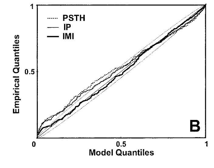
Figure 1 from : the time-rescaling Q–Q plot for a neural spike train model. Points within the confidence bands indicate a good fit. — Figure 1 from Brown *et al.*, 2002: the time-rescaling Q–Q plot for a neural spike train model. Points within the confidence bands indicate a good fit.

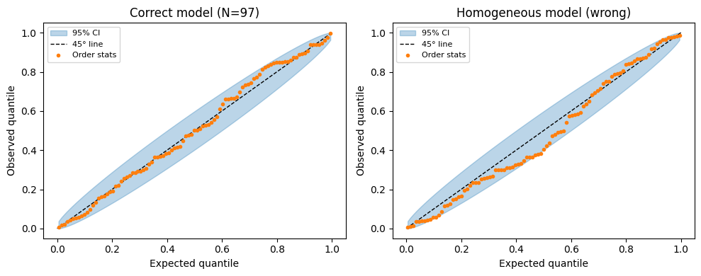
np.random.seed(0)

# True process: inhomogeneous PP with lambda(t) = 2 + sin(pi*t/5)
T_gof = 50.0
def true_intensity(t):
    return 2.0 + np.sin(np.pi * t / 5.0)

def cum_intensity(t):
    # Lambda(t) = 2t - (5/pi)*cos(pi*t/5) + 5/pi
    return 2.0 * t - (5.0 / np.pi) * np.cos(np.pi * t / 5.0) + 5.0 / np.pi

# Sample events via thinning
lam_max_gof = 3.1
events_np = sample_pp_thinning(true_intensity, lam_max_gof, T_gof).numpy()
N_obs = len(events_np)

def gof_plot(ax, events, intensity_fn, cum_intensity_fn, T, title):
    '''KS / time-rescaling goodness-of-fit Q-Q plot.'''
    xs = np.sort(events)
    # compute Lambda differences
    xs_with_zero = np.concatenate([[0.0], xs])
    Lambda_vals = np.array([cum_intensity_fn(t) for t in xs_with_zero])
    Delta = np.diff(Lambda_vals)
    z = 1 - np.exp(-Delta)
    z_sorted = np.sort(z)
    n_pts = len(z_sorted)
    ns = np.arange(1, n_pts + 1)
    expected = (ns - 0.5) / n_pts
    # Beta confidence bands
    lower = beta_dist.ppf(0.025, ns, n_pts - ns + 1)
    upper = beta_dist.ppf(0.975, ns, n_pts - ns + 1)
    ax.fill_between(expected, lower, upper, alpha=0.3, color='tab:blue', label='95% CI')
    ax.plot([0, 1], [0, 1], 'k--', lw=1, label='45° line')
    ax.plot(expected, z_sorted, 'o', ms=3, color='tab:orange', label='Order stats')
    ax.set_xlabel('Expected quantile')
    ax.set_ylabel('Observed quantile')
    ax.set_title(title)
    ax.legend(fontsize=8)

fig, axes = plt.subplots(1, 2, figsize=(10, 4))

# Good fit: use the true intensity
gof_plot(axes[0], events_np, true_intensity, cum_intensity,
         T_gof, f'Correct model (N={N_obs})')

# Poor fit: use a constant (wrong) rate
lam_wrong = N_obs / T_gof
def cum_wrong(t):
    return lam_wrong * t
gof_plot(axes[1], events_np, lambda t: lam_wrong, cum_wrong,
         T_gof, f'Homogeneous model (wrong)')

plt.tight_layout()
plt.savefig('gof_demo.png', dpi=100, bbox_inches='tight')
plt.show()

Hawkes Processes¶

Hawkes processes Hawkes, 1971 are self-exciting point processes whose conditional intensity depends on the history of past events.

The conditional intensity is,

\lambda(t \mid \mathcal{H}_t) = \lambda_0 + \sum_{t_n \in \mathcal{H}_t} h(t - t_n),

(7)

where $h: \mathbb{R}_+ \to \mathbb{R}_+$ is a non-negative impulse response (or influence function) and $\mathcal{H}_t = \{t_n : t_n < t\}$ is the history up to time $t$ .

A common choice is an exponential impulse response,

h(\Delta t) = \frac{w}{\tau} e^{-\Delta t / \tau} = w \cdot \mathrm{Exp}(\Delta t;\, \tau),

(8)

where $\tau > 0$ is the time constant and $w > 0$ is the total weight (i.e., the expected number of events triggered per event, $\int_0^\infty h(\Delta t)\, d(\Delta t) = w$ ).

Maximum Likelihood Estimation¶

The Hawkes log-likelihood has the same form as the Poisson process likelihood,

\log p(\{t_n\} \mid \theta) = -\int_0^T \lambda_\theta(t \mid \mathcal{H}_t)\, dt + \sum_{n=1}^N \log \lambda_\theta(t_n \mid \mathcal{H}_{t_n}).

(9)

With an exponential impulse response and parameters $\theta = (\lambda_0, w)$ , this simplifies to,

\log p \approx -\theta^\top \phi_0 + \sum_{n=1}^N \log(\theta^\top \phi_n),

(10)

where $\phi_0 = (T, N)^\top$ and $\phi_n = \big(1,\; \sum_{t_m < t_n} \mathrm{Exp}(t_n - t_m;\, \tau)\big)^\top$ .

Multivariate Hawkes Processes¶

A multivariate Hawkes process Linderman & Adams, 2014 models $S$ interacting sources with mutually excitatory interactions,

\lambda_s(t \mid \mathcal{H}_t) = \lambda_{s,0} + \sum_{(t_n, s_n) \in \mathcal{H}_t} h_{s_n, s}(t - t_n),

(11)

where $h_{s,s'}(\Delta t)$ is a directed impulse response from source $s$ to source $s'$ .

The weights $\mathbf{W}$ with $W_{s,s'} = \int_0^\infty h_{s,s'}(\Delta t)\, d(\Delta t)$ define a directed network of interactions.

Example from : inferred network structure from a multivariate Hawkes process fit to neural spike train data. — Example from Linderman & Adams, 2014: inferred network structure from a multivariate Hawkes process fit to neural spike train data.

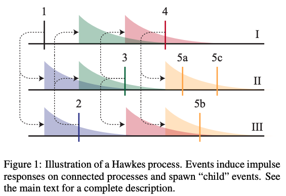
Hawkes Processes as Poisson Clustering¶

By the superposition principle, the points from each source $s$ can be decomposed into clusters:

\mathcal{T}_s = \mathcal{T}_{s,0} \cup \bigcup_{n=1}^N \mathcal{T}_{s,n},

(12)

where $\mathcal{T}_{s,0} \sim \mathrm{PP}(\lambda_{s,0})$ are background events and $\mathcal{T}_{s,n} \sim \mathrm{PP}(h_{s_n, s}(t - t_n))$ are events triggered by the $n$ -th event. With exponential impulse responses, $\mathbb{E}[|\mathcal{T}_{s,n}|] = w_{s_n, s}$ .

This clustering representation enables a Gibbs sampler for Bayesian inference: with a Gamma prior $w_{s,s'} \sim \mathrm{Ga}(\alpha, \beta)$ , the weights and cluster assignments have conjugate conditionals that can be sampled alternately.

def sample_hawkes(lam0, w, tau, T, seed=0):
    '''Sample a univariate Hawkes process with exponential impulse response.

    Args:
        lam0: baseline intensity
        w: excitation weight (expected offspring per event)
        tau: time constant of exponential impulse response
        T: end of interval
        seed: random seed
    Returns:
        sorted numpy array of event times
    '''
    rng = np.random.default_rng(seed)
    events = []
    t = 0.0
    # Use Ogata's thinning algorithm
    while t < T:
        # Upper bound on intensity given current history
        lam_bar = lam0 + (w / tau) * sum(np.exp(-(t - ti) / tau) for ti in events)
        # Next candidate event
        dt = rng.exponential(1.0 / lam_bar)
        t_cand = t + dt
        if t_cand > T:
            break
        # Evaluate true intensity at candidate
        lam_cand = lam0 + (w / tau) * sum(np.exp(-(t_cand - ti) / tau) for ti in events)
        # Accept/reject
        if rng.uniform() < lam_cand / lam_bar:
            events.append(t_cand)
        t = t_cand
    return np.array(sorted(events))


T_hawkes = 100.0
events_hawkes = sample_hawkes(lam0=1.0, w=0.6, tau=1.0, T=T_hawkes, seed=7)
N_hawkes = len(events_hawkes)

# Plot: event raster + conditional intensity
ts_h = np.linspace(0, T_hawkes, 2000)
tau_h = 1.0
lam0_h = 1.0
w_h = 0.6
lam_t = np.array([
    lam0_h + (w_h / tau_h) * sum(np.exp(-(t - ti) / tau_h) for ti in events_hawkes if ti < t)
    for t in ts_h
])

fig, axes = plt.subplots(2, 1, figsize=(12, 5), sharex=True)
axes[0].fill_between(ts_h, lam_t, alpha=0.4, color='tab:red')
axes[0].plot(ts_h, lam_t, color='tab:red', lw=0.8)
axes[0].axhline(lam0_h, ls='--', color='k', lw=0.8, label=r'$\lambda_0$')
axes[0].set_ylabel(r'$\lambda(t \mid \mathcal{H}_t)$')
axes[0].set_title(f'Hawkes process: $\lambda_0={lam0_h}$, $w={w_h}$, $\tau={tau_h}$ — {N_hawkes} events')
axes[0].legend()

axes[1].eventplot(events_hawkes, lineoffsets=0.5, linelengths=0.8, color='k')
axes[1].set_xlabel('Time')
axes[1].set_ylabel('Events')
axes[1].set_yticks([])
axes[1].set_xlim(0, T_hawkes)
axes[1].set_ylim(0, 1)

plt.tight_layout()
plt.savefig('hawkes_demo.png', dpi=100, bbox_inches='tight')
plt.show()
print(f"Average rate: {N_hawkes / T_hawkes:.2f} (expected: {lam0_h / (1 - w_h):.2f})")

<>:53: SyntaxWarning: invalid escape sequence '\l'
<>:53: SyntaxWarning: invalid escape sequence '\l'
/tmp/ipykernel_2805/3277385441.py:53: SyntaxWarning: invalid escape sequence '\l'
  axes[0].set_title(f'Hawkes process: $\lambda_0={lam0_h}$, $w={w_h}$, $\tau={tau_h}$ — {N_hawkes} events')

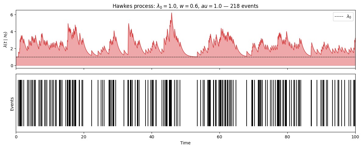
Average rate: 2.18 (expected: 2.50)

Doubly Stochastic (Cox) Processes¶

Hawkes processes introduce dependence through the past. An alternative is to model the intensity itself as a random process — these are called doubly stochastic processes or Cox processes.

In these models,

\lambda(\mathbf{x}) \sim p(\lambda),

(13)

and then, given $\lambda$ , the points are generated as a Poisson process with that intensity.

Log Gaussian Cox process: Let $f \sim \mathrm{GP}(\mu(\cdot), K(\cdot, \cdot))$ and set $\lambda(\mathbf{x}) = e^{f(\mathbf{x})}$ . This gives a flexible, non-negative intensity with a log-Gaussian marginal distribution at each point.

Sigmoidal Gaussian Cox process Adams et al., 2009: Use $\lambda(\mathbf{x}) = \sigma(f(\mathbf{x})) \cdot \lambda_{\max}$ where $\sigma$ is the sigmoid function. This allows exact inference via a thinning construction.

Neyman–Scott process Wang et al., 2022: Let $\lambda$ be a convolution of a Poisson process with a non-negative kernel. This generates clustered point patterns where events arise in groups.

The key challenge in all these models is computing (or approximating) the intractable integral $\int \lambda(\mathbf{x})\, d\mathbf{x}$ in the likelihood.

Summary¶

Poisson processes are defined by an intensity function $\lambda(\mathbf{x})$ and two properties: Poisson counts and independence of disjoint sets.
They can be sampled by four methods: top-down, intervals (homogeneous), time-rescaling, and thinning (rejection sampling).
The time-rescaling theorem yields a simple goodness-of-fit test: if the model is correct, the rescaled intervals are i.i.d. $\mathrm{Exp}(1)$ , and after a further transformation, the order statistics fall along a 45° line.
Hawkes processes introduce self-excitation via a conditional intensity that depends on past events; their clustering representation enables efficient Bayesian inference.
Cox processes introduce dependence by modeling the intensity as a stochastic process, typically a Gaussian process transformed to be non-negative.

References¶

Brown, E. N., Barbieri, R., Ventura, V., Kass, R. E., & Frank, L. M. (2002). The time-rescaling theorem and its application to neural spike train data analysis. Neural Computation, 14(2), 325–346.
Hawkes, A. G. (1971). Spectra of some self-exciting and mutually exciting point processes. Biometrika, 58(1), 83–90.
Linderman, S., & Adams, R. (2014). Discovering latent network structure in point process data. International Conference on Machine Learning, 1413–1421.
Adams, R. P., Murray, I., & MacKay, D. J. (2009). Tractable nonparametric Bayesian inference in Poisson processes with Gaussian process intensities. Proceedings of the 26th Annual International Conference on Machine Learning, 9–16.
Wang, Y., Degleris, A., Williams, A. H., & Linderman, S. W. (2022). Spatiotemporal Clustering with Neyman-Scott Processes via Connections to Bayesian Nonparametric Mixture Models. arXiv Preprint arXiv:2201.05044.