Exponential Families#
Many familiar distributions like the ones we covered in lecture 1 are exponential family distributions. As Brad Efron likes to say, exponential family distributions bridge the gap between the Gaussian family and general distributions. For Gaussian distributions, we have exact small-sample distributional results (\(t\), \(F\), and \(\chi^2\) tests); in the exponential family setting we have approximate distributional results (deviance tests); in the general setting, we have to appeal to asymptotics.
import torch
import matplotlib.pyplot as plt

from torch.distributions import Poisson, Normal
from torch.distributions.kl import kl_divergence
Definition#
Exponential family distributions have densities of the form,
where
\(h(y): \cY \to \reals_+\) is the base measure,
\(t(y) \in \reals^T\) are the sufficient statistics,
\(\eta \in \reals^T\) are the natural parameters, and
\(A(\eta): \reals^T \to \reals\) is the log normalizing function (aka the partition function).
The log normalizer ensures that the density is properly normalized,
The domain of the exponential family is the set of valid natural parameters, \(\Omega = \{\eta: A(\eta) < \infty\}\). An exponential family is a family of distributions defined by base measure \(h\) and sufficient statistics \(t\), and it is indexed by natural paremeters \(\eta \in \Omega\).
Examples#
Gaussian with known variance#
Consider the scalar Gaussian distribution,
We can write this as an exponential family distribution where, where
the base measure is \(h(y) = \frac{e^{-\frac{y^2}{2 \sigma^2}}}{\sqrt{2 \pi \sigma^2}}\)
the sufficient statistics are \(t(y) = \frac{y}{\sigma}\)
the natural parameter is \(\eta = \frac{\mu}{\sigma}\)
the log normalizer is \(A(\eta) = \frac{\eta^2}{2}\)
the domain is \(\Omega = \reals\)
Poisson distribution#
Likewise, take the Poisson pmf,
where
the base measure is \(h(y) = \frac{1}{y!}\)
the sufficient statistics are \(t(y) = y\)
the natural parameter is \(\eta = \log \lambda\)
the log normalizer \(A(\eta) = \lambda = e^\eta\)
the domain is \(\Omega = \reals\)
Bernoulli distribution#
Exercise
Write the Bernoulli distribution in exponential family form. Recall that its pmf is
What are the base measure, the sufficient statistics, the natural parameter, the log normalizer, and the domain?
Categorical distribution#
Finally, take the categorical pmf for \(Y \in \{1, \ldots, K\}\),
where
the base measure is \(h(y) = \bbI[y \in \{1,\ldots,K\}]\)
the sufficient statistics are \(t(y) = \mbe_y\), the one-hot vector representation of \(y\)
the natural parameter is \(\mbeta = \log \mbpi = (\log \pi_1, \ldots, \log \pi_K)^\top \in \reals^K\)
the log normalizer \(A(\mbeta) = 0\)
the domain is \(\Omega = \reals^K\)
The Log Normalizer#
The cumulant generating function — i.e., the log of the moment generative function — is a difference of log normalizers,
Its derivatives (with respect to \(\theta\) and evaluated at zero) yield the cumulants. In particular,
\(\nabla_\theta K_\eta(0) = \nabla A(\eta)\) yields the first cumulant of \(t(Y)\), its mean
\(\nabla^2_\theta K_\eta(0) = \nabla^2 A(\eta)\) yields the second cumulant, its covariance
Higher order cumulants can be used to compute skewness, kurtosis, etc.
Gradient of the log normalizer#
We can also obtain this result more directly.
Again, the gradient of the log normalizer yields the expected sufficient statistics,
Hessian of the log normalizer#
The Hessian of the log normalizer yields the covariance of the sufficient statistics,
Maximum Likelihood Estimation#
Suppose we have \(y_i \iid\sim p(y; \eta)\) for a minimal exponential family distribution with natural parameter \(\eta\). The log likelihood is,
The gradient is
and the Hessian is \(\nabla^2 \cL(\eta) = -n \nabla^2 A(\eta)\).
Since the log normalizer is convex, all local optima are global. If the log normalizer is strictly convex, the MLE will be unique.
Setting the gradient to zero and solving yields the stationary conditions for the MLE,
When \(\nabla A\) is invertible, the MLE is unique,
Even if \(\nabla A\) is not invertible, maximum likelihood estimation amounts to matching empirical means of the sufficient statistics to corresponding natural parameters.
Asymptotic normality#
Recall that the MLE is asymptotically normal with variance given by the inverse Fisher information,
Thus, the asymptotic covariance of \(\hat{\eta}_{\mathsf{MLE}}\) is \(\cI(\eta)^{-1} = \tfrac{1}{n} \Cov_\eta[t(Y)]^{-1}\).
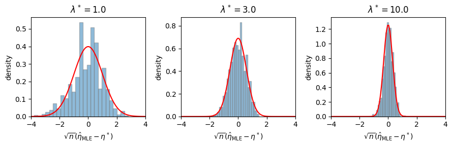
Example: MLE for the Poisson distribution#
Suppose \(Y_i \iid{\sim} \mathrm{Po}(\lambda)\) for \(i=1,\ldots,n\). The natural parameter of the Poisson distribution is \(\eta = \log \lambda\), and the maximum likelihood estimate is \(\hat{\eta}_{\mathsf{MLE}} = \log \left(\frac{1}{n} \sum_{i=1}^n y_i \right)\). The Fisher information matrix is the variance, \(\cI(\eta) = \mathrm{Var}_\eta[Y] = e^\eta\).
# Simulate a Poisson and look at the distribution of the MLE
def sample_and_compute_mle(seed, n, lmbda_true):
    torch.manual_seed(seed)
    ys = Poisson(lmbda_true).sample((n,))
    eta_mle = torch.log(ys.mean())
    return eta_mle

# Compute the MLE for a range of true rates
lmbda_trues = torch.tensor([1.0, 3.0, 10.0])
fig, axs = plt.subplots(1, len(lmbda_trues), figsize=(3 * len(lmbda_trues), 3))
n = torch.as_tensor(30)
for ax, lmbda_true in zip(axs, lmbda_trues):
    eta_true = torch.log(lmbda_true)
    fisher_info = Poisson(lmbda_true).variance

    mles = torch.tensor([sample_and_compute_mle(seed, n, lmbda_true) for seed in range(1000)])

    # Plot a histogram of the MLEs alongside the asymptotic normal distribution
    etas = torch.linspace(-4, 4, 100)
    ax.hist(torch.sqrt(n) * (mles - eta_true), density=True, bins=25, alpha=0.5, edgecolor='gray')
    ax.plot(etas, Normal(0, torch.sqrt(1 / fisher_info)).log_prob(etas).exp(), color='red')
    ax.set_xlim(-4, 4)
    ax.set_xlabel(r"$\sqrt{n}(\hat{\eta}_{\mathsf{MLE}} - \eta^*)$")
    ax.set_ylabel(r"density")
    ax.set_title(rf"$\lambda^* = {lmbda_true}$")

plt.tight_layout()
Minimal Exponential Families#
The Hessian of the log normalizer gives the covariance of the sufficient statistic. Since covariance matrices are positive semi-definite, the log normalizer is a convex function on \(\Omega\).
If the covariance is strictly positidive definite — i.e., if the minimum eigenvalue of \(\nabla^2 A(\eta)\) is strictly greater than zero for all \(\eta \in \Omega\) — then the log normalizer is strictly convex. In that case, we say that the exponential family is minimal
Question
Is the exponential family representation of the categorical distribution above a minimal representation? If not, how could you encode it in minimal form?
Answer
The categorical representation above is not minimal because the log normalizer is identically zero, and hence it is not strictly convex. The problem stems from the fact that the natural parameters \(\mbeta \in \reals^K\) include log probabilities for each of the \(K\) classes, whereas the probabilities \(\mbpi \in \Delta_{K-1}\) must sum to one, and thus really lie in a \(K-1\) dimensional simplex.
Instead, we could parameterize the categorical distribution in terms of the log probabilities for only the first \(K-1\) classes,
where
the base measure is \(h(y) = \bbI[y \in \{1,\ldots,K\}]\)
the sufficient statistics are \(\mbt(y) = (\bbI[y=1], \ldots, \bbI[y=K-1])^\top\)
the natural parameter is \(\mbeta = (\eta_1, \ldots, \eta_{K-1})^\top \in \reals^{K-1}\) where \(\eta_k = \log \frac{\pi_k}{1 - \sum_{j=1}^{K-1} \pi_j}\) are the logits
the log normalizer \(A(\mbeta) = \log \left(1 + \sum_{k=1}^{K-1} e^{\eta_k} \right)\)
the domain is \(\Omega = \reals^{K-1}\)
Mean Parameterization#
When constructing models with exponential family distributions, like the generalized linear models below, it is often more convenient to work with the mean parameters instead. for a \(d\)-dimensional sufficient statistic, let,
denote the set of mean parameters realizable by any distribution \(p\).
Two facts:
The gradient mapping \(\nabla A: \Omega \mapsto \cM\) is injective (one-to-one) if and only if the exponential family is minimal.
The gradient is a surjective mapping from mean parameters to the interior of \(\cM\). All mean parameters in the interior of \(\cM\) (excluding the boundary) can be realized by an exponential family distribution. (Mean parameters on the boundary of \(\cM\) can be realized by a limiting sequence of exponential family distributions.)
Together, these facts imply that the gradient of the log normalizer defines a bijective map from \(\Omega\) to the interior of \(\cM\) for minimal exponential families.
For minimal families, we can work with the mean parameterization instead,
for mean parameters \(\mu\) in the interior of \(\cM\).
MLE for the Mean Parameters#
Alternatively, consider the maximum likelihood estimate of the mean parameter \(\mu \in \cM\). Before doing any math, we might expect the MLE to be the empirical mean. Indeed, that is the case. To simplify notation, let \(\eta(\mu) = [\nabla A]^{-1}(\mu)\). The log likelihood,
has gradient,
where \(\tfrac{\partial \eta}{\partial \mu}(\mu)\) is the Jacobian of inverse gradient mapping at \(\mu\). Assuming the Jacobian is positive definite, we immediately see that,
Now back to the Jacobian… applying the inverse function theorem, shows that it equals the inverse covariance matrix,
which is indeed positive definite for minimal exponential families.
Asymptotic normality#
We obtain the Fisher information of the mean parameter \(\mu\) by left and right multiplying by the Jacobian,
Thus, the MLE of the mean parameter is asymptotically normal with covariance determined by the inverse Fisher information, \(\cI(\mu)^{-1} = \Cov_{\eta(\mu)}[t(Y)]\). More formally,
As usual, to derive confidence intervals we plug in the MLE to evaluate the asymptotic covariance.
Note
Compare this result to the asymptotic covariances we computed in Lecture 1 for the Bernoulli distribution. Recall that for \(X_i \iid\sim \mathrm{Bern}(\theta)\), where \(\theta \in [0,1]\) is the mean parameter, we found,
Now we see that this is a general property of exponential family distributions.
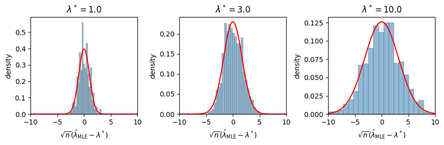
Revisiting the Poisson example#
Revisiting the example above, here we have \(\hat{\lambda}_{\mathsf{MLE}} = \frac{1}{n} \sum_i y_i\) and \(\cI(\lambda) = \mathrm{Var}_\lambda[Y]^{-1} = \frac{1}{\lambda}\). We expect,
# Simulate a Poisson and look at the distribution of the MLE
def sample_and_compute_mle(seed, n, lmbda_true):
    torch.manual_seed(seed)
    ys = Poisson(lmbda_true).sample((n,))
    lmbda_mle = ys.mean()
    return lmbda_mle

# Compute the MLE for a range of true rates
lmbda_trues = torch.tensor([1.0, 3.0, 10.0])
fig, axs = plt.subplots(1, len(lmbda_trues), figsize=(3 * len(lmbda_trues), 3))
n = torch.as_tensor(30)
for ax, lmbda_true in zip(axs, lmbda_trues):
    fisher_info = 1 / Poisson(lmbda_true).variance

    mles = torch.tensor([sample_and_compute_mle(seed, n, lmbda_true) for seed in range(1000)])

    # Plot a histogram of the MLEs alongside the asymptotic normal distribution
    lmbdas = torch.linspace(-10, 10, 100)
    ax.hist(torch.sqrt(n) * (mles - lmbda_true), density=True, bins=25, alpha=0.5, edgecolor='gray')
    ax.plot(lmbdas, Normal(0, torch.sqrt(1 / fisher_info)).log_prob(lmbdas).exp(), color='red')
    ax.set_xlim(-10, 10)
    ax.set_xlabel(r"$\sqrt{n} (\hat{\lambda}_{\mathsf{MLE}} - \lambda^*)$")
    ax.set_ylabel(r"density")
    ax.set_title(rf"$\lambda^* = {lmbda_true}$")

plt.tight_layout()
Conjugate duality#
The log normalizer is a convex function. Its conjugate dual is,
We recognize this as the maximum likelihood problem mapping expected sufficient statistics \(\mu\) to natural parameters \(\eta\). For minimal exponential families, the supremum is uniquely obtained at \(\eta(\mu) = [\nabla A]^{-1}(\mu)\). The conjugate dual evaluates to the log likelihood obtained at \(\eta(\mu)\).
It turns out the conjugate dual is also related to the entropy; in particular, for any \(\mu\) in the interior of \(\cM\),
where \(\eta(\mu) = [\nabla A]^{-1}(\mu)\) for minimal exponential families. To see this, note that
Moreover, for minimal exponential families, the gradient of \(A^*\) provides the inverse map from mean parameters to natural parameters,
Finally, the log normalizer has a variataional representation in terms of its conjugate dual,
For more on conjugate duality, see Wainwright and Jordan [WJ08], ch. 3.6.
KL Divergence#
The Kullback-Leibler (KL) divergence, or relative entropy, between two distributions is,
It is non-negative and equal to zero if and only if \(p = q\). The KL divergence is not a distance because it is not a symmetric function of \(p\) and \(q\). (generally, \(\KL{p}{q} \neq \KL{q}{p}\).)
When \(p\) and \(q\) belong to the same exponential family with natural parameters \(\eta_p\) and \(\eta_q\), respectively, the KL simplifies to,
This form highlights that the KL divergence between exponential family distributions is a special case of a Bregman divergence based on the convex function \(A\).
Example: Poisson Distribution
Consider the Poisson distribution with known mean \(\lambda\). In the example above, we cast it as an exponential family distribution with
sufficient statistics \(t(y) = y\)
natural parameter \(\eta = \log \lambda\)
log normalizer \(A(\eta) = e^\eta\)
Derive the KL divergence between two Poisson distributions with means \(\lambda_p\) and \(\lambda_q\), respectively.
Answer
The KL divergence is,
Example: Gaussian Distribution
Consider the scalar Gaussian distribution with known variance \(\sigma^2\). In the example above, we cast it as an exponential family distribution with
sufficient statistics \(t(y) = \frac{y}{\sigma}\)
natural parameter \(\eta = \frac{\mu}{\sigma}\)
log normalizer \(A(\eta) = \frac{\eta^2}{2}\)
Derive the KL divergence between two Gaussians with equal variance. Denote their natural parameters by \(\eta_p = \frac{\mu_p}{\sigma}\) and \(\eta_q = \frac{\mu_q}{\sigma}\), respectively.
Answer
The KL divergence is,
Note that here, the KL is a symmetric function.
Deviance#
Rearranging terms, we can view the KL divergence as a remainder in a Taylor approximation of the log normalizer,
From this perspective, we see that the KL divergence is related to the Fisher information,
up to terms of order \(\cO(\|\eta_p - \eta_q\|^3)\).
Thus, while the KL divergence is not a distance metric due to its asymmetry, it is approximately a squared distance under the Fisher information metric,
We call this quantity the deviance. It is simply twice the KL divergence.
Deviance Residuals#
In a normal model, the standarized residual is \(\frac{\hat{\mu} - \mu}{\sigma}\). We can view this as a function of the deviance between two normals,
where we have used the shorthand notation
The same form generalizes to other exponential families as well, with the deviance residual between the true and estimated mean parameters defined as,
One can show that deviance residuals tend to be closer to normal than the more obvious Pearson residuals,
For more on deviance residuals, see Efron [Efr22], ch. 1.
Revisiting the Poisson example#
Finally, let’s revisit the Poisson example one again. We already computed the KL divergence between two Poisson distributions above,
so the deviance residual is,
Compare this to the Pearon residual,
Let’s compare these residuals in simulation.
# Simulate a Poisson and compute deviance and Pearson residuals
def sample_and_compute_residuals(seed, n, lmbda_true):
    torch.manual_seed(seed)
    ys = Poisson(lmbda_true).sample((n,))
    lmbda_mle = ys.mean()
    deviance_residuals = torch.sign(lmbda_mle - lmbda_true) \
        * torch.sqrt(2 * kl_divergence(Poisson(lmbda_mle), Poisson(lmbda_true)))
    pearson_residuals = (lmbda_mle - lmbda_true) / torch.sqrt(lmbda_mle)
    return deviance_residuals, pearson_residuals

# Compute the MLE for a range of true rates
lmbda_trues = torch.tensor([0.5, 1.0, 10.0])
fig, axs = plt.subplots(2, len(lmbda_trues), figsize=(3 * len(lmbda_trues), 6), sharex=True, sharey=True)
n = torch.as_tensor(20)
lim = 1.5
rs = torch.linspace(-lim, lim, 100)
for k, lmbda_true in enumerate(lmbda_trues):
    residuals = [sample_and_compute_residuals(seed, n, lmbda_true) for seed in range(1000)]
    deviance_residuals, pearson_residuals = zip(*residuals)

    # Plot a histogram of the MLEs alongside the asymptotic normal distribution
    axs[0,k].hist(deviance_residuals, density=True, bins=30, alpha=0.5, edgecolor='gray', label="deviance")
    axs[0,k].plot(rs, Normal(0, 1 / torch.sqrt(n)).log_prob(rs).exp(), color='red')
    axs[0,k].set_xlim(-lim, lim)
    axs[0,k].set_xlabel(r"deviance residual")
    axs[0,k].set_ylabel(r"density")
    axs[0,k].set_title(rf"$\lambda^* = {lmbda_true}$")

    axs[1,k].hist(pearson_residuals, density=True, bins=30, alpha=0.5, edgecolor='gray', label="pearson")
    axs[1,k].plot(rs, Normal(0, 1 / torch.sqrt(n)).log_prob(rs).exp(), color='red')
    axs[1,k].set_xlim(-lim, lim)
    axs[1,k].set_xlabel(r"Pearson residual")
    axs[1,k].set_ylabel(r"density")

plt.tight_layout()
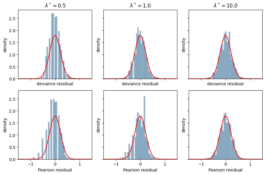
Note that I considered \(\lambda^* \in [0.5, 1, 10]\) instead of \([1,3,10]\) to see if differences were exaggerated at smaller rates. My intuitions was that we might not expect big differences when the rates are reasonably large, since in that regime the Poisson starts to look fairly Gaussian. Here, however, it’s hard for me to say which residual is better — by eye, they look pretty similar. If you check out Brad’s book, you can see that there are indeed differences that suggest deviance residuals are better behaved, it’s just not so evident in this example.
Conclusion#
Exponential family distributions have many beautiful properties, and we’ve only scratched the surface in this chapter.
We’ll see other nice properties when we talk about building probabilistic models for joint distributions of random variables using exponential family distributions, and conjugate relationships between exponential families will simplify many aspects of Bayesian inference.
We’ll also see that inference in exponential families is closely connected to convex optimization — we saw that today for the MLE! — but for more complex models, the optimization problems can still be computationally intractable, even though its convex. That will motivate our discussion of variational inference later in the course.
Armed with exponential family distributions, we can start to build more expressive models for categorical data. First up, generalized linear models!