Basics of Probability and Statistics

This lecture introduces the basic building blocks that we’ll use throughout the course. We start with common distributions for discrete random variables. Then we discuss some basics of statistical inference: maximum likelihood estimation, asymptotic normality, hypothesis tests, confidence intervals, and Bayesian inference.

Big Picture

This course is about probabilistic modeling and inference with discrete data.

What is the end goal?

• Predict: given features, estimate labels or outputs

• Simulate: given partial observations, generate the rest

• Summarize: given high dimensional data, find low-dimensional factors of variation

• Decide: given past actions/outcomes, which choice is best?

• Understand: what generative mechanisms gave rise to this data?

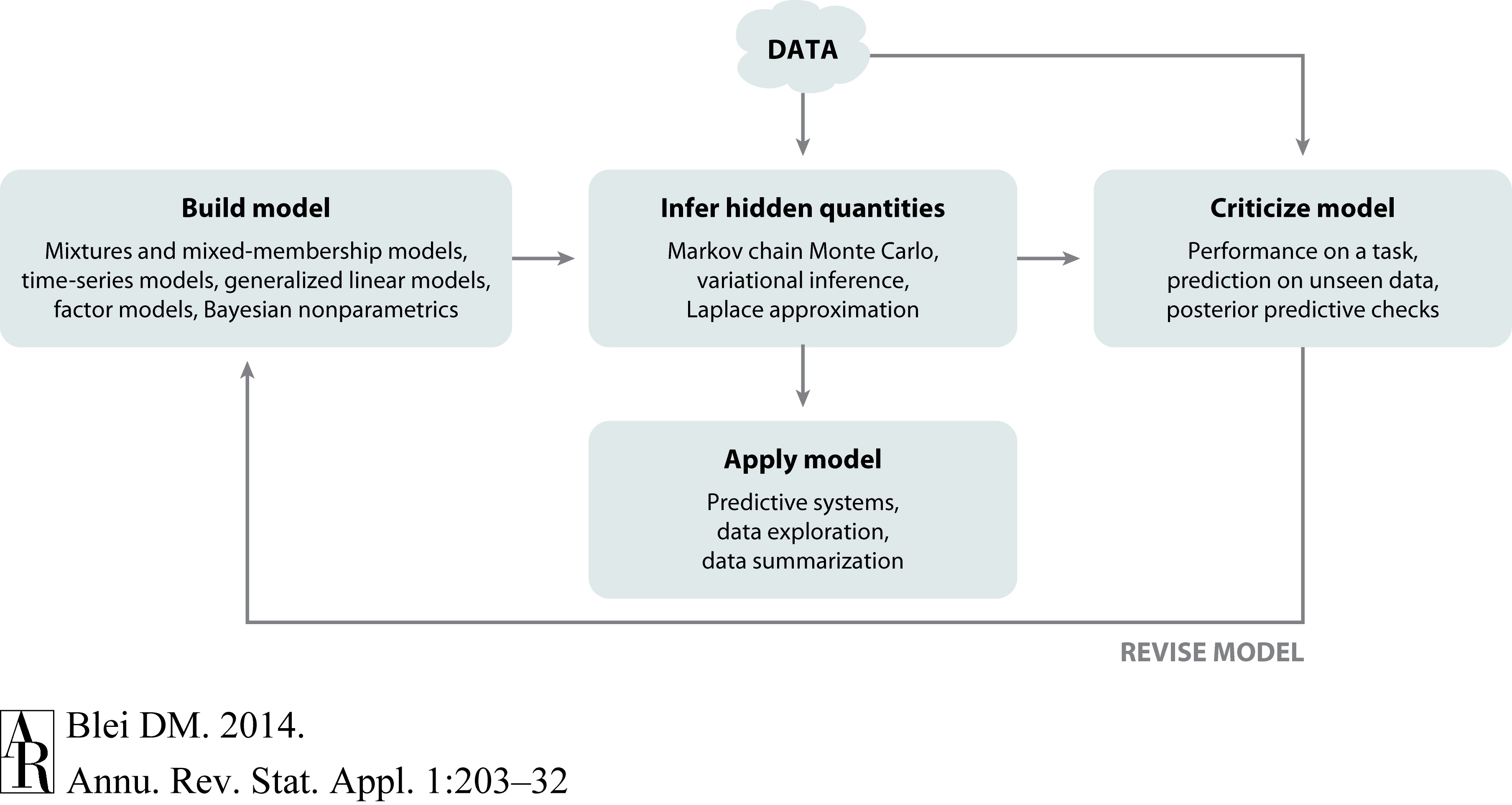
Box’s Loop

Bernoulli Distribution

Toss a (biased) coin where the probability of heads is \(p \in [0,1]\). Let \(X=1\) denote the event that a coin flip comes up heads and \(X=0\) it comes up tails. The random variable \(X\) follows a Bernoulli distribution,

\[\begin{align*} X \sim \mathrm{Bern}(p) \end{align*}\]

We denote its probability mass function (pmf) by,

\[\begin{align*} \mathrm{Bern}(x; p) = \begin{cases} p & \text{if } x = 1 \\ 1 - p &\text{if } x = 0 \end{cases} \end{align*}\]

or more succinctly

\[\begin{align*} \mathrm{Bern}(x; p) = p^x (1-p)^{1-x}. \end{align*}\]

(We will use this mildly overloaded nomenclature to represent both the distribution \(\mathrm{Bern}(p)\) and its pmf \(\mathrm{Bern}(x; p)\). The difference will be clear from context.)

The Bernoulli distribution’s mean is \(\E[X] = p\) and its variance is \(\Var[X] = p(1-p)\).

Binomial Distribution

Now toss the same biased coin \(n\) times independently and let

\[\begin{align*} X_i &\iid\sim \mathrm{Bern}(p) & \text{for } i&=1,\ldots, n \end{align*} \]

denote the outcomes of each trial.

The number of heads, \(X = \sum_{i=1}^n X_i\), is a random variable taking values \(X \in \{0,\ldots,n\}\). It follows a binomial distribution,

\[\begin{align*} X \sim \mathrm{Bin}(n, p) \end{align*}\]

with pmf

\[\begin{align*} \mathrm{Bin}(x; n, p) = {n \choose x} p^x (1-p)^{n-x}. \end{align*}\]

Its mean and variance are \(\E[X] = np\) and \(\Var[X] = np(1-p)\), respectively.

Poisson Distribution

Now let \(n \to \infty\) and \(p \to 0\) while the product \(np = \lambda\) stays constant. For example, instead of coin flips, suppose we’re modeling spikes fired by a neuron in a 1 second interval of time. For simplicity, assume we divide the 1 second interval into \(n\) equally sized bins, each of width \(1/n\) seconds. Suppose probability of seeing at least one spike in a bin is proportional to the bin width, \(p=\lambda / n\), where \(\lambda \in \reals_+\) is the rate. (For now, assume \(\lambda < n\) so that \(p < 1\).) Moreover, suppose each bin is independent. Then the number of bins with at least one spike is binomially distributed,

\[\begin{align*} X \sim \mathrm{Bin}(n, \lambda / n). \end{align*}\]

Intuitively, the number of bins shouldn’t really matter — it just determines our resolution for detecting spikes. We really care about is the number of spikes, which is separate from the binning process. As \(n \to \infty\), the number of spikes in the unit interval converges to a Poisson random variable,

\[\begin{align*} X \sim \mathrm{Po}(\lambda). \end{align*}\]

Its pmf is,

\[\begin{align*} \mathrm{Po}(x; \lambda) &= \frac{1}{x!} e^{-\lambda} \lambda^x. \end{align*}\]

Its mean and variance are both \(\lambda\). The fact that the mean equals the variance is a defining property of the Poisson distribution, but it’s not always an appropriate modeling assumption. We’ll discuss more general models shortly.

Categorical Distribution

So far, we’ve talked about distributions for scalar random variables. Here, we’ll extend these ideas to vectors of counts.

Instead of a biased coin, consider a biased die with \(K\) faces and corresponding probabilites \(\mbpi = (\pi_1, \ldots, \pi_K) \in \Delta_{K-1}\), where

\[\begin{align*} \Delta_{K-1} &= \left\{\mbpi \in \reals_+^K: \sum_k \pi_k = 1 \right\} \end{align*}\]

denotes the \((K-1)\)-dimensional simplex embedded in \(\reals^K\).

Roll the die and let the random variable \(X \in \{1,\ldots,K\}\) denote the outcome. It follows a categorical distribution,

\[\begin{align*} X &\sim \mathrm{Cat}(\mbpi) \end{align*}\]

with pmf

\[\begin{align*} \mathrm{Cat}(x; \mbpi) &= \prod_{k=1}^K \pi_k^{\bbI[x=k]} \end{align*}\]

where \(\bbI[y]\) is an indicator function that returns 1 if \(y\) is true and 0 otherwise. This is a natural generalization of the Bernoulli distribution to random variables that can fall into more than two categories.

Alternatively, we can represent \(X\) as a one-hot vector, in which case \(X \in \{\mbe_1, \ldots, \mbe_K\}\) where \(\mbe_k = (0, \ldots, 1, \ldots, 0)^\top\) is a one-hot vector with a 1 in the \(k\)-th position. Then, the pmf is,

\[\begin{align*} \mathrm{Cat}(\mbx; \mbpi) &= \prod_{k=1}^K \pi_k^{x_k} \end{align*}\]

Multinomial Distribution

From this representation, it is straightforward to generalize to \(n\) independent rolls of the die, just like in the binomial distribution. Let \(Z_i \iid\sim \mathrm{Cat}(\mbpi)\) for \(i=1,\ldots,n\) denote the outcomes of each roll, and let \(X = \sum_{i=1}^n Z_i\) denote the total number of times the die came up on each of the \(K\) faces. Note that \(X \in \naturals^K\) is a vector-valued random variable. Then, \(X\) follows a multinomial distribution,

\[\begin{align*} X \sim \mathrm{Mult}(n, \mbpi), \end{align*}\]

with pmf,

\[\begin{align*} \mathrm{Mult}(\mbx; n, \mbpi) &= \bbI[\mbx \in \cX_n] \cdot {n \choose x_1, \ldots , x_K} \prod_{k=1}^K \pi_k^{x_k} \end{align*}\]

where \(\cX_n = \left\{\mbx \in \naturals^K : \sum_{k=1}^K x_k = n \right\}\) and

\[\begin{align*} {n \choose x_1, \ldots, x_K} &= \frac{n!}{x_1! \cdots x_K!} \end{align*}\]

denotes the multinomial function.

The expected value of a multinomial random variable is \(\E[X] = n \mbpi\) and the \(K \times K\) covariance matrix is,

\[\begin{align*} \Cov(X) &= n \begin{bmatrix} \pi_1(1-\pi_1) & -\pi_1 \pi_2 & \ldots & -\pi_1 \pi_K \\ -\pi_2 \pi_1 & \pi_2 (1-\pi_2) & \ldots & -\pi_2 \pi_K \\ \vdots & \vdots & \vdots & \vdots \\ -\pi_K \pi_1 & -\pi_K \pi_2 & \ldots & \pi_K (1- \pi_K) \end{bmatrix} \end{align*}\]

with entries

\[\begin{align*} [\Cov[X]]_{ij} &= \begin{cases} n \pi_i (1-\pi_i) & \text{if } i = j \\ -n \pi_i \pi_j & \text{if } i \neq j \\ \end{cases} \end{align*}\]

Poisson / Multinomial Connection

Suppose we have a collection of independent (but not identically distributed) Poisson random variables,

\[\begin{align*} X_i &\sim \mathrm{Po}(\lambda_i) & \text{for } i&=1,\ldots,K. \end{align*}\]

Due to their independence, the sum \(X_\bullet = \sum_{i=1}^K X_i\) is Poisson distributed as well,

\[\begin{align*} X_\bullet &\sim \mathrm{Po}\left( \sum_{i=1}^K \lambda_k \right) \end{align*}\]

(We’ll use this \(X_\bullet\) notation more next time.)

Conditioning on the sum renders the counts dependent. (They have to sum to a fixed value, so they can’t be independent!) Specifically, given the sum, the counts follow a multinomial distribution,

\[\begin{align*} (X_1, \ldots, X_K) \mid X_\bullet = n &\sim \mathrm{Mult}(n, \mbpi) \end{align*}\]

where

\[\begin{align*} \mbpi &= \left(\frac{\lambda_1}{\lambda_\bullet}, \ldots, \frac{\lambda_K}{\lambda_\bullet} \right) \end{align*}\]

with \(\lambda_{\bullet} = \sum_{i=1}^K \lambda_i\). In words, given the sum, the vector of counts is multinomially distributed with probabilities given by the normalized rates.

Maximum Likelihood Estimation

The distributions above are simple probability models with one or two parameters. How can we estimate those parameters from data? We’ll focus on maximum likelihood estimation.

The log likelihood is the probability of the data viewed as a function of the model parameters \(\mbtheta\). Given i.i.d. observations \(\{x_i\}_{i=1}^n\), the log likelihood reduces to a sum,

\[\begin{align*} \cL(\mbtheta) &= \sum_{i=1}^n \log p(x_i; \theta). \end{align*}\]

The maximum likelihood estimate (MLE) is a maximum of the log likelihood,

\[\begin{align*} \hat{\mbtheta}_{\mathsf{MLE}} &= \arg\; \max \cL(\mbtheta) \end{align*}\]

(Assume for now that there is a single global maximum.)

Example: MLE for the Bernoulli distribution

Consider a Bernoulli distribution unknown parameter \(\theta \in [0,1]\) for the probability of heads. Suppose we observe \(n\) independent coin flips

\[\begin{align*} X_i &\iid\sim \mathrm{Bern}(\theta) & \text{for } i&=1,\ldots, n. \end{align*}\]

Observing \(X_i=x_i\) for all \(i\), the log likelihood is,

\[\begin{align*} \cL(\theta) &= \sum_{i=1}^n x_i \log \theta + (1 - x_i) \log (1 - \theta) \\ &= x \log \theta + (n - x) \log (1 - \theta) \end{align*}\]

where \(x = \sum_{i=1}^n x_i\) is the number of flips that came up heads.

Taking the derivative with respect to \(p\),

\[\begin{align*} \frac{\dif}{\dif \theta} \cL(\theta) &= \frac{x}{\theta} - \frac{n - x}{1 - \theta} \\ &= \frac{x - n\theta}{\theta (1 - \theta)}. \end{align*}\]

Setting this to zero and solving for \(\theta\) yields the MLE,

\[\begin{align*} \hat{\theta}_{\mathsf{MLE}} = \frac{x}{n}. \end{align*}\]

Intuitively, the maximum likelihood estimate is the fraction of coin flips that came up heads. Note that we could have equivalently expressed this model as a single observation of \(X \sim \mathrm{Bin}(n, \theta)\) and obtained the same result.

Asymptotic Normality of the MLE

If the data were truly generated by i.i.d. draws from a model with parameter \(\mbtheta^\star\), then under certain conditions the MLE is asymptotically normal and achieves the Cramer-Rao lower bound,

\[\begin{align*} \sqrt{n} (\hat{\mbtheta}_{\mathsf{MLE}} - \mbtheta^\star) \to \cN(0, \cI(\mbtheta^\star)^{-1}) \end{align*}\]

in distribution, where \(\cI(\mbtheta)\) is the Fisher information matrix. We obtain standard error estimates by taking the square root of the diagonal elements of the inverse Fisher information matrix and dividing by \(\sqrt{n}\).

Fisher Information Matrix

The Fisher information matrix is the covariance of the score function, the partial derivative of the log likelihood with respect to the parameters. It’s easy to confuse yourself with poor notation, so let’s try to derive it precisely.

The log probability is a function that maps two arguments (a data point and a parameter vector) to a scalar, \(\log p: \cX \times \Theta \mapsto \reals\). The score function is the partial derivative with respect to the parameter vector, which is itself a function, \(\nabla_\theta \log p: \cX \times \Theta \mapsto \Theta\).

Now consider \(\mbtheta\) fixed and treat \(X \sim p(\cdot; \mbtheta)\) as a random variable. The expected value of the score is zero,

\[\begin{align*} \E_{X \sim p(\cdot; \mbtheta)}[\nabla_\theta \log p(X; \mbtheta)] &= \int_{\cX} p(x; \mbtheta) \nabla_\theta \log p (x; \mbtheta) \dif x \\ &= \int_{\cX} p(x; \mbtheta) \frac{\nabla_\theta p(x; \mbtheta)}{p(x; \mbtheta)} \dif x \\ &= \nabla_\theta \int_{\cX} p(x; \mbtheta) \dif x \\ &= \nabla_\theta 1 \\ &= \mbzero. \end{align*}\]

The Fisher information matrix is the covariance of the score function, again treating \(\mbtheta\) as fixed,

\[\begin{align*} \cI(\mbtheta) &= \Cov_{X \sim p(\cdot; \mbtheta)}[\nabla_\theta \log p(X; \mbtheta)] \\ &= \E_{X \sim p(\cdot; \mbtheta)}[\nabla_\theta \log p(X; \mbtheta) \nabla_\theta \log p(X; \mbtheta)^\top] - \underbrace{\E_{X \sim p(\cdot; \mbtheta)}[\nabla_\theta \log p(X; \mbtheta)]}_{\mbzero} \, \underbrace{\E_{X \sim p(\cdot; \mbtheta)}[\nabla_\theta \log p(X; \mbtheta)]^\top}_{\mbzero^\top} \\ &= \E_{X \sim p(\cdot; \mbtheta)}[\nabla_\theta \log p(X; \mbtheta) \nabla_\theta \log p(X; \mbtheta)^\top]. \end{align*}\]

If \(\log p\) is twice differentiable (in \(\mbtheta\)) the under certain regularity conditions, the Fisher information matrix is equivalent to the expected value of the negative Hessian of the log probability,

\[\begin{align*} \cI(\mbtheta) &= - \E_{X \sim p(\cdot; \mbtheta)}\left[ \nabla_\mbtheta^2 \log p (X; \mbtheta) \right] \end{align*}\]

Example: Fisher Information for the Bernoulli Distribution

For a Bernoulli distribution, the log probability and its score were evaluated above,

\[\begin{align*} \log p(x; \theta) &= x \log \theta + (1 - x) \log (1 - \theta) \\ \nabla_\theta \log p(x; \theta) &= \frac{x - \theta}{\theta (1 - \theta)} \end{align*}\]

The negative Hessian with respect to \(\theta\) is,

\[\begin{align*} - \nabla^2_\theta \log p(x; \theta) &= \frac{x}{\theta^2} + \frac{1 - x}{(1 - \theta)^2}. \end{align*}\]

Taking the expectation w.r.t. \(X \sim p(\cdot; \theta)\) yields,

\[\begin{align*} \cI(\theta) &= -\E\left[\nabla^2_\theta \log p(x; \theta) \right] \\ &= \frac{\theta}{\theta^2} + \frac{1- \theta}{(1-\theta)^2} \\ &= \frac{1}{\theta (1 - \theta)}. \end{align*}\]

Interestingly, the inverse Fisher information is the \(\Var[X; \theta]\). We’ll revisit this point when we discuss exponential family distributions.

Hypothesis Testing

Suppose we want to test a null hypothesis \(\cH_0: \theta = \theta_0\) for a scalar parameter \(\theta \in \reals\). Exploiting the asymptotic normality of the MLE, the test statistic,

\[\begin{align*} z &= \frac{\hat{\theta} - \theta_0}{\sqrt{\cI(\hat{\theta})^{-1} / n}} \end{align*}\]

approximately follows a standard normal distribution under the null hypothesis. From this we can derive one- or two-sided p-values. (We dropped the \(\mathsf{MLE}\) subscript on \(\hat{\theta}\) to simplify notation.)

Wald test

Equivalently,

\[\begin{align*} z^2 &= \frac{(\hat{\theta} - \theta_0)^2}{\cI(\hat{\theta})^{-1} / n} \end{align*}\]

has a chi-squared null distribution with 1 degree of freedom. When the non-null standard error derived from the Fisher information at \(\hat{\theta}\) is used to compute the test statistic, it is called a Wald statistic.

For multivariate settings, \(\cH_0: \mbtheta = \mbtheta_0\) with \(\mbtheta \in \reals^D\), the Wald statistic generalizes to,

\[\begin{align*} z^2 &= (\hat{\mbtheta} - \mbtheta_0)^\top [\cI(\hat{\mbtheta})^{-1} / n]^{-1} (\hat{\mbtheta} - \mbtheta_0) \\ &= n (\hat{\mbtheta} - \mbtheta_0)^\top \cI(\hat{\mbtheta}) (\hat{\mbtheta} - \mbtheta_0), \end{align*}\]

which has a chi-squared null distribution with \(D\) degrees of freedom. The p-value is then the probability of seeing a value at least as large as \(z^2\) under the chi-squared distribution.

Wald tests are one of the three canonical large-sample tests. The other two are the likelihood ratio test and the score test (a.k.a., the Lagrange multiplier test). Asymptotically, they are equivalent, but in finite samples they differ. See Agresti [Agr02] (Sec 1.3.3) for more details.

Confidence Intervals

In practice, we often care more about estimating confidence intervals for parameters than testing specific hypotheses about their values. Given a hypothesis test with level \(\alpha\), like the Wald test above, we can construct a confidence interval with level \(1-\alpha\) by taking all \(\theta\) for which \(\cH_0\) has a p-value exceeding \(\alpha\).

For example, a 95% Wald confidence interval for a scalar parameter is the set,

\[\begin{align*} \left\{\theta_0: \frac{|\hat{\theta} - \theta_0|}{\sqrt{\cI(\hat{\theta})^{-1} / n}} < 1.96 \right\} &= \hat{\theta} \pm 1.96 \sqrt{\cI(\hat{\theta})^{-1} / n} \end{align*}\]

Equivalent confidence intervals can be derived from the tails of the chi-squared distribution. Note that the confidence interval is a function of the observed data from which the MLE is computed.

Example: Confidence Intervals for a Bernoulli Parameter

Continuing our running example, we found that the MLE of a Bernoulli parameter is \(\hat{\theta} = x/n\) and the inverse Fisher information is \(\cI(\theta)^{-1} = \theta (1 - \theta)\). Together, these yield a 95% Wald confidence interval of,

\[\begin{align*} \hat{\theta} \pm 1.96 \sqrt{\frac{\hat{\theta} ( 1 - \hat{\theta})}{n}}. \end{align*}\]

Again, this should be intuitive. If we were estimating the mean of a Gaussian distribution, the variance of the estimator would scale be roughly \(1/n\) times the variance of an individual observation. Since \(\hat{\theta} ( 1 - \hat{\theta})\) is the variance of a Bernoulli distribution with parameter \(\hat{\theta}\), we see similar behavior here.

Conclusion

That’s it! We’ve had our first taste of models and algorithms for discrete data. It may seem like a stretch to call a basic distribution a “model,” but that’s exactly what it is. Likewise, the procedures we derived for computing the MLE of a Bernoulli distribution, and constructing Wald confidence intervals are our first “algorithms.” These will be our building blocks as we construct more sophisticated models and algorithms for more complex data.