HW0: PyTorch Primer#
STATS305B, Stanford University, Winter 2025
Your name:
Collaborators:
Hours spent:
Please let us know how many hours in total you spent on this assignment so we can calibrate for future assignments. Your feedback is always welcome!
We’ll use Python and PyTorch for the assignments in this course. This lab is to help you get up to speed. It will introduce:
Tensors: PyTorch’s equivalent of NumPy arrays, but with more bells and whistles for running on GPUs and supporting automatic differentiation.
Broadcasting and Fancy Indexing: If you’re coming from Matlab or NumPy, you probably know that you can avoid costly for-loops by broadcasting computation over dimensions of an array (here, tensor) and using fancy indexing tricks.
Distributions: PyTorch has an excellent library of distributions for sampling, evaluating log probabilities, and much more.
import torch
import torch.distributions as dist
import matplotlib.pyplot as plt
1. Constructing Tensors#
Tensors are PyTorch’s equivalent of NumPy arrays. The PyTorch documentation already has a great tutorial on tensors. Rather than recreate the wheel, please start by reading that.
Once you’ve read through that, try using torch functions like arange, reshape, etc. to construct the following tensors.
Problem 1.1#
Construct the following tensor:
tensor([[0, 1, 2],
        [3, 4, 5],
        [6, 7, 8]])
Note: For this problems and the ones below, don’t literally construct the tensor from the specified list. Use torch functions.
# YOUR CODE HERE
Problem 1.2#
Construct the following tensor:
tensor([[0, 3, 6],
        [1, 4, 7],
        [2, 5, 8]])
# YOUR CODE HERE
Problem 1.3#
Construct the following tensor:
tensor([0, 1, 2, 3, 4, 0, 1, 2, 3, 4, 0, 1, 2, 3, 4])
Note: Here the sequence is repeated 3 times. Does your code support arbitrary numbers of repeats?
# YOUR CODE HERE
Problem 1.4#
Construct the following tensor:
tensor([[0, 1, 2, 3, 4],
        [0, 1, 2, 3, 4],
        [0, 1, 2, 3, 4]])
# YOUR CODE HERE
Problem 1.5#
Construct the following tensor:
tensor([[ 1., -2.,  0.,  0.],
        [-2.,  1., -2.,  0.],
        [ 0., -2.,  1., -2.],
        [ 0.,  0., -2.,  1.]])
# YOUR CODE HERE
Problem 1.6#
Construct the following tensor:
tensor([[[[0, 1, 2]]]])
# YOUR CODE HERE
2. Broadcasting and Fancy Indexing#
Your life will be much easier and your code will be much faster once you get the hang of broadcasting and indexing. Start by reading the PyTorch documentation.
Problem 2.1#
Construct a tensor X where X[i,j] = i + j by broadcasting a sum of two 1-dimensional tensors.
For example, broadcast a sum to construct the following tensor,
tensor([[0, 1, 2],
        [1, 2, 3],
        [2, 3, 4],
        [3, 4, 5]])
# YOUR CODE HERE
Problem 2.2#
Compute a distance matrix D where D[i,j] is the Euclidean distance between X[i] and X[j], with
X = torch.arange(10, dtype=float).reshape(5, 2)
Your answer should be,
tensor([[ 0.0000,  2.8284,  5.6569,  8.4853, 11.3137],
        [ 2.8284,  0.0000,  2.8284,  5.6569,  8.4853],
        [ 5.6569,  2.8284,  0.0000,  2.8284,  5.6569],
        [ 8.4853,  5.6569,  2.8284,  0.0000,  2.8284],
        [11.3137,  8.4853,  5.6569,  2.8284,  0.0000]])
X = torch.arange(10, dtype=float).reshape(5, 2)
# YOUR CODE HERE
Problem 2.3#
Extract the submatrix of rows [2,3] and columns [0,1,4] of the tensor,
A = torch.arange(25).reshape(5, 5)
Your answer should be,
tensor([[10, 11, 14],
        [15, 16, 19]])
A = torch.arange(25).reshape(5, 5)
# YOUR CODE HERE
Problem 2.4#
Create a binary mask matrix M of the same shape as A where M[i,j] is True if and only if A[i,j] is divisible by 7. Let
A = torch.arange(25).reshape(5, 5)
Your answer should be
tensor([[ True, False, False, False, False],
        [False, False,  True, False, False],
        [False, False, False, False,  True],
        [False, False, False, False, False],
        [False,  True, False, False, False]])
A = torch.arange(25).reshape(5, 5)
# YOUR CODE HERE
Problem 2.5#
Add one to the entries in A that are divisible by 7. After updating in place, A should be,
tensor([[ 1,  1,  2,  3,  4],
        [ 5,  6,  8,  8,  9],
        [10, 11, 12, 13, 15],
        [15, 16, 17, 18, 19],
        [20, 22, 22, 23, 24]])
# YOUR CODE HERE
3. Distributions#
PyTorch has an excellent library of distributions in torch.distributions. Read the docs here.
We will use these distribution objects to construct and fit a Poisson mixture model.
Problem 3.1#
Draw 50 samples from a Poisson distribution with rate 10.
# YOUR CODE HERE
Problem 3.2#
One of the awesome thing about PyTorch distributions is that they support broadcasting too.
Construct a matrix P where P[i,j] equals \(\mathrm{Pois}(x=j; \lambda=i)\) for \(i=0,\ldots,4\) and \(j=0,\ldots,4\).
Your answer should be,
tensor([[1.0000, 0.0000, 0.0000, 0.0000, 0.0000],
        [0.3679, 0.3679, 0.1839, 0.0613, 0.0153],
        [0.1353, 0.2707, 0.2707, 0.1804, 0.0902],
        [0.0498, 0.1494, 0.2240, 0.2240, 0.1680],
        [0.0183, 0.0733, 0.1465, 0.1954, 0.1954]])
# YOUR CODE HERE
Problem 3.3#
Evaluate the log probability of the points [1.5, 3., 4.2] under a gamma distribution with shape (aka concentration) 2.0 and inverse scale (aka rate) 1.5.
Your answer should be,
tensor([-1.0336, -2.5905, -4.0540])
# YOUR CODE HERE
Problem 3.4#
Draw 1000 samples from a Poisson mixture model,
Use matplotlib.pyplot.hist to plot a normalized histogram of the samples.
# YOUR CODE HERE
# data = ...
4. PyTorch Distributions#
Problem 4.1#
Use dist.Normal to draw a batch of shape (100, 4) independent standard normal random variables.
# YOUR CODE HERE
Problem 4.2#
Use dist.Normal to draw a batch independent normal random variables with shape (5,5), variance 1.0, and means
tensor([[ 0,  1,  2,  3,  4],
        [ 5,  6,  8,  8,  9],
        [10, 11, 12, 13, 15],
        [15, 16, 17, 18, 19],
        [20, 22, 22, 23, 24]])
# YOUR CODE HERE
5. Debugging#
“If debugging is the process of removing bugs, then programming must be the process of putting them in.” -Edsger Dijkstra
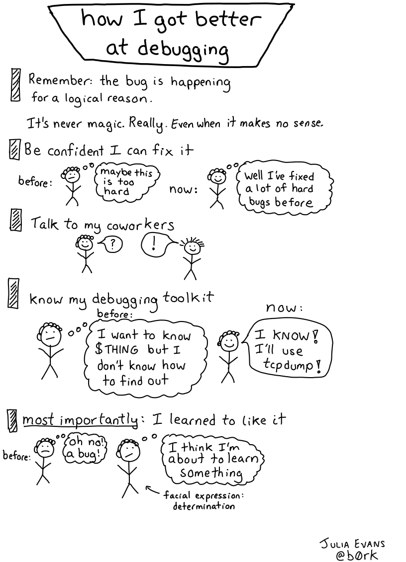
Debugging is an important skill in applied statistics that we will hone in this class. The following exercises will introduce you to useful python debugging tools and techniques.
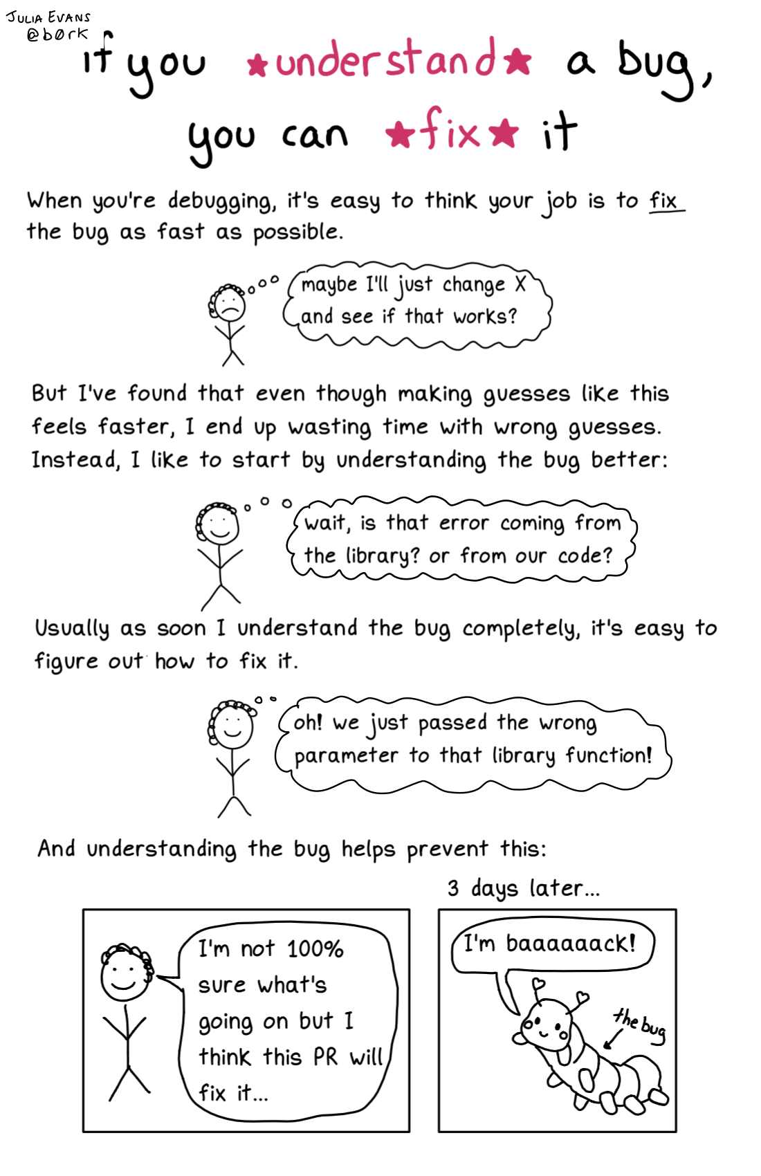
In particular, we will focus on giving you some tools that let you more directly interrogate what is happening in a code snippet. Hopefully, learning how to understand what is going on in a given code snippet will replace feelingness of powerlessness when encountering an inscrutable bug with confidence, mastery, and knowledge.
Problem 5.1: sleuthing with type, shape, and dir#
Many python bugs effectively arise from errors in grammar—trying to apply functions to objects in ways that don’t make sense based on the type or shape of the object.
For example, in English, you can’t say: “I enjoy to beautiful the park,” because you have put an adjective (“beautiful”) where a verb belongs. In a similar way, you can’t evalaute the python expression "number:" + 7, because the + operator has different actions for strings and for ints.
So, when you encounter an unfamiliar object in the course of writing python code, instead of throwing spaghetti at the wall and seeing what sticks, it can be helpful to get to know the object better, in particular by asking what its type and, if applicable, shape is, as well as what attributes it has. This approach is similar how you might get to know a new friend, by asking the name, where the person is from, what the person does—you would not start by randomly guessing different names for a new person!
Problem 5.1.1#
What is the type of "number:"? What is the type of 7? What is the type of A from Problem 2.4?
Use the type function explicitly to answer this question.
# TODO: your code and answers here
Problem 5.1.2#
What are the shapes of "number:" and 7 and A? Can you give an intuitive reason why some types have shapes and other don’t?
Call .shape on the above objects explicitly to answer this question
# TODO: your code and answers here
Problem 5.1.3#
Call dir on the three objects
"number:7A
Describe what you notice. For each of the three objects, try out one of the methods that you get from calling dir. Does it have the behavior you would expect from the name? Describe why or why not.
# TODO: your code and answers here
Problem 5.2: pdb#
Problem 5.2.1: %debug#
The % denotes a magic command, which opens up commands that are not in standard python, but are added by IPython, which is short for “Interactive Python” and is the backbone of JuPyter notebooks and colabs.
If you run a cell that returns an Error, in the very next cell you can just type %debug and then run the cell (Shft + Enter), and you open up a python debugger at the very point where the error was raised. Then, you can interactively investigate the values (as well as types and shapes) of the variables that were in and before the line that led to the crash. You can navigate through the debugger with these commands
Try running the following code (which has a bug). When it errors out, run %debug in the next cell. In the ipd> console, find the shapes of both tensor_a and tensor_b by asking for their shape, and explain why the code does’t work. Exit the debugger with quit().
# BUGGY CODE
tensor_a = torch.randn(2, 2)
tensor_b = torch.randn(3, 2)
result = tensor_a @ tensor_b
Problem 5.2.2: breakpoint()#
Sometimes the bug can be more subtle, either not causing any error messages or having the bug be introduced many lines before the error is raised. In these situations, it can be helpful to add a breakpoint() to your code.
Add a breakpoint() anywhere to the code snippet in Problem 5.2.1, and confirm that you can still print types, shapes, and values, and navigate using pdb commands.
Problem 5.3: Debugging Linear Regression#
Below is some buggy code for fitting linear regression on synthetic data that we will use to practice other debugging techniques
#BUGGY CODE
# generate synthetic data
torch.manual_seed(305)
n = 100_000
p = 3
X = torch.hstack([torch.ones((n,1)), torch.randn(n, p)])
beta_true = torch.randn(p+1)
y = X @ beta_true + torch.randn(n)

# set up logistic regression
loss_fn = torch.nn.MSELoss()
beta_hat = torch.randn(p+1, requires_grad=True)

learning_rate = 2.
num_iterations = 100

losses = []
# Gradient Descent
for i in range(num_iterations):
    # Forward pass
    y_pred = X @ beta_hat

    # Compute and print loss
    loss = loss_fn(y_pred, y)
    losses.append(loss.item())

    # Zero the gradients before running the backward pass
    beta_hat.grad = None

    # Backward pass
    loss.backward()

    # Update weights using gradient descent
    with torch.no_grad():
        beta_hat += (learning_rate / (i+1)) * beta_hat.grad

# The final parameters after training
beta_final = beta_hat.detach()
Problem 5.3.1: assert and torch.allclose#
In the above code snippet, we would like to recover the true value beta_true of the linear regression coefficients in our final value beta_final. One way to check if two vectors are close each other is to use torch.allclose, which will return True if the two vectors have each corresponding element within atol of each other. One way to do this programatically is with an assert, which raises an error if the condition following it not true.
Edit the above code snippet by adding an assert which checks if beta_true and beta_final are within a margin of 1e-2 elementwise.
Problem 5.3.2: f-strings#
It can be useful for debugging to print output, which can be done very cleanly using f-strings (the “f” stands for “formatted”). In particular, the second argument to an assert (after the boolean expression) can be a string that is printed if the boolean is False.
Modify your assert so that if beta_true and beta_final are not true, their values are printed with a descrption of what they are, using f-strings for easy comparison.
Problem 5.3.3: plotting#
Use matplotlib.pyplot, which was imported in the very first cell as plt, to plot the lossess in the above code snippet. What do you notice about the losses? Does this clue you into the location of the bug? Fix the bug in the code snippet above.
Problem 5.3.4: progress bars#
It’s extremely nice to know how long code is going to take to run. One easy way to add this is to wrap for loops (like in the above code snippet) with progress bars. Probably the easiest way to do this is with the tqdm package, which can be as as easy as:
from tqdm import tqdm

for i in tqdm(range(10)):
  print(i)
Add a progress bar to the above code snippet.
Problem 5.3.5: timing#
Often you want your code to run quickly when you are prototyping. How might you modify the above code snippet to run faster when you are just prototyping? Note that because you are “prototyping,” your “quick-and-dirty” solution doesn’t need to satisfy the asserts you set up in Problem 5.3.1.
But, DO confirm that your approach is faster by using %%time. Report your findings.
TODO: your summary of your timing experiments
6. More resources#
An excellent 1-unit introduction to Python. Meets Wednesdays 11:30-12:30 in winter quarter. Strongly recommend concurrent enrollment if you are new to python.
An excellent introduction to software tools. While not directly related to Stats 305B, the tools reviewed in this series will make you a more confident programmer.
7. Submission Instructions#
Formatting: check that your code does not exceed 80 characters in line width. You can set Tools → Settings → Editor → Vertical ruler column to 80 to see when you’ve exceeded the limit.
Converting to PDF The simplest way to convert to PDF is to use the “Print to PDF” option in your browser. Just make sure that your code and plots aren’t cut off, as it may not wrap lines.
Alternatively You can download your notebook in .ipynb format and use the following commands to convert it to PDF. Then run the following command to convert to a PDF:
jupyter nbconvert --to pdf <yourlastname>_hw<number>.ipynb
(Note that for the above code to work, you need to rename your file <yourlastname>_hw<number>.ipynb)
Installing nbconvert:
If you’re using Anaconda for package management,
conda install -c anaconda nbconvert
Upload your .pdf file to Gradescope. Please tag your questions correctly! I.E., for each question, all of and only the relevant sections are tagged.
Please post on Ed or come to OH if there are any other problems submitting the HW.