Gaussian Processes#
Week 8 is about Bayesian nonparametrics and stochastic processes, starting with Gaussian processes. This notebook is a demo relating a Bayesian linear regression with RBF features to a squared exponential kernel.
import torch
import matplotlib.pyplot as plt
# Pull the data from HW 1
!wget -nc https://raw.githubusercontent.com/slinderman/stats305c/main/assignments/hw1/hw1.pt
Xs, ys = torch.load("hw1.pt")

# Recall that X is a (N, 2) tensor where the first column is all ones
# We just want the x locations (the second column)
xs = Xs[:, 1]
zsh:1: command not found: wget
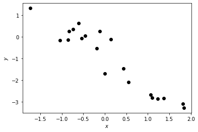
# Plot the data
plt.plot(xs, ys, 'ko')
plt.xlabel("$x$")
plt.ylabel("$y$")
Text(0, 0.5, '$y$')
Linear regression with RBF basis functions#
Let’s start with a Bayesian linear regression using an RBF feature encoding,
with center \(c_p\) and width \(\ell\). The model was,
where
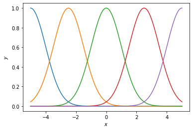
First, let’s look at the basis with different numbers of basis functions.
# Set up a finite RBF basis
def rbf(x, center, length_scale):
    return torch.exp(-0.5 / length_scale**2 * (x - center)**2)

def plot_basis(num_basis, xlim=5, length_scale=1.0):
    centers = torch.linspace(-xlim, xlim, num_basis)
    x_grid = torch.linspace(-xlim, xlim, 500)
    for center in centers:
        plt.plot(x_grid, rbf(x_grid, center, length_scale))

    plt.xlabel("$x$")
    plt.ylabel("$y$")
plot_basis(5)
plot_basis(10)
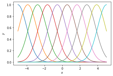
Now fit a linear regression with this basis#
We will first compute the posterior \(p(\mathbf{w} \mid \{x_n, y_n\}_{n=1}^N)\), then we’ll use it to predict \(y_{N+1}\) for a grid of points \(x_{N+1}\).
def fit_rbf_regression(xs, ys,
                       xlim=5,
                       num_basis=10,
                       length_scale=1.0,
                       prior_var=1.0,
                       lkhd_var=0.5**2):
    """Fit a Bayesian linear regression with an RBF feature encoding.

    Parameters
    ----------
    xs, ys: 1D inputs and outputs of the regression
    xlim: max absolute value of the RBF centers
    num_basis: number of RBF features, evenly spaced between +/-xlim
    length_scale: length_scale of the RBF kernels
    prior_var: prior variance of the weights
    lkhd_var: variance of the likelihood y ~ N(w \cdot \phi(x), sigma^2)
    """
    centers = torch.linspace(-xlim, xlim, num_basis)

    # Encode the data in the RBFs.
    encoded_xs = rbf(xs[:, None], centers[None, :], length_scale)

    # Assuming fixed and likelihood variances, compute the posterior
    # distribution of the weights
    J_post = num_basis / prior_var * torch.eye(num_basis) \
           + encoded_xs.T @ encoded_xs / lkhd_var
    h_post = encoded_xs.T @ ys / lkhd_var
    Sigma_post = torch.linalg.inv(J_post)
    mu_post = Sigma_post @ h_post

    # Compute the predictive mean at a dense grid of points
    x_grid = torch.linspace(-xlim, xlim, 100)
    encoded_grid = rbf(x_grid[:, None], centers[None, :], length_scale)
    mu_pred = encoded_grid @ mu_post
    Sigma_pred = encoded_grid @ Sigma_post @ encoded_grid.T \
        + lkhd_var * torch.eye(100)

    # Plot the mean and +-3 standard deviations of the posterior
    for i in range(1, 4):
        plt.fill_between(x_grid,
                        mu_pred - i * torch.sqrt(torch.diag(Sigma_pred)),
                        mu_pred + i * torch.sqrt(torch.diag(Sigma_pred)),
                        color='r', alpha=0.1)
    plt.plot(x_grid, mu_pred, '-r', lw=3)
    plt.plot(xs, ys, 'o')
    plt.xlabel("$x$")
    plt.xlim(-xlim, xlim)
    plt.ylabel("$y$")
fit_rbf_regression(xs, ys, num_basis=5)
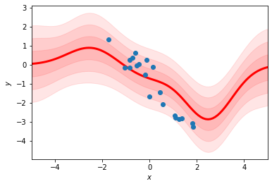
fit_rbf_regression(xs, ys, num_basis=10)

fit_rbf_regression(xs, ys, num_basis=20)
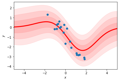
Questions#
Why are the mean and variance of the predictions more “wiggly” in the first plot?
Why do the predicted means decay back to zero as \(|x|\) increases rather than following the linear trend of the data?
What would happen if we increased the prior variance?
What would happen if we increased the likelihood variance?
Now use a Gaussian process with a squared exponential kernel#
In class we introduced the squared exponential kernel
with variance \(\varsigma^2\) and length scale \(\ell'\). We showed how it arises from Bayesian linear regression with an encoding into an infinite set of radial basis functions. Concretely, the squared exponential kernel with variance \(\varsigma^2 = \sqrt{\pi} \ell \lambda\) and length scale \(\ell' = \sqrt{2} \ell\) is the infinite limit of the RBF regression.
def fit_sqexp_gp(xs, ys,
                 length_scale=1.0,
                 prior_var=1.0,
                 lkhd_var=0.5**2,
                 xlim=5.0):
    N = len(xs)

    # Define the squared exponential kernel function. Account for the scaling
    # constants necessary to equate with the RBF regression
    def kernel(x_i, x_j):
        scale = 0.1 * torch.sqrt(torch.tensor(torch.pi)) * length_scale * prior_var
        return scale * torch.exp(-0.5 / (torch.sqrt(torch.tensor(2)) * \
                                         length_scale)**2 * (x_i - x_j)**2)

    # Compute the Gram matrix
    K = kernel(xs[:, None], xs[None, :])

    # Compute the predictive mean at a dense grid of points
    x_grid = torch.linspace(-xlim, xlim, 1000)
    K_grid = kernel(xs[:, None], x_grid[None, :])

    K_chol = torch.linalg.cholesky(K + lkhd_var * torch.eye(N))
    mu_pred = K_grid.T @ torch.cholesky_solve(ys[:, None], K_chol)[:, 0]
    Sigma_pred = kernel(x_grid[:, None], x_grid[None, :]) \
        - K_grid.T @ torch.cholesky_solve(K_grid, K_chol) + lkhd_var * torch.eye(1000)

    # Plot the mean and +-3 standard deviations of the posterior
    for i in range(1, 4):
        plt.fill_between(x_grid,
                         mu_pred - i * torch.sqrt(torch.diag(Sigma_pred)),
                         mu_pred + i * torch.sqrt(torch.diag(Sigma_pred)),
                         color='r', alpha=0.1)
    plt.plot(x_grid, mu_pred, '-r', lw=3)
    plt.plot(xs, ys, 'o')
    plt.xlabel("$x$")
    plt.xlim(-xlim, xlim)
    plt.ylabel("$y$")

fit_sqexp_gp(xs, ys)

Comparison to the RBF regression#
This should look like the RBF regression as we take the number of basis functions to infinity.
fit_rbf_regression(xs, ys, num_basis=100)

Questions#
What happens if you increase the prior variance?
What happens if you decrease the likelihood variance?
What happens if you decrease the length scale?
GP Classification with a Probit Mean Function#
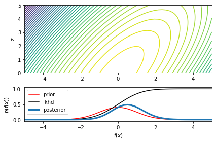
First, let’s visualize the joint distribution over \(f(x)\) and \(z\), assuming
# Make a g
xlim = 5
x_grid = torch.linspace(-xlim, xlim, 50)
z_grid = torch.linspace(0, xlim, 50)
XX, ZZ = torch.meshgrid(x_grid, z_grid)

# Compute the log joint probability
lp_xz = torch.distributions.Normal(0, 1).log_prob(XX)
lp_xz += torch.distributions.Normal(XX, 1).log_prob(ZZ)
lp_xz -= torch.logsumexp(lp_xz, (0, 1))
# p_xz = torch.exp(lp_xz)

# Compute the marginal
lp_x = torch.logsumexp(lp_xz, axis=1)
lp_x -= (torch.logsumexp(lp_x, 0) + torch.log(x_grid[1] - x_grid[0]))
lp_x_prior = torch.distributions.Normal(0, 1).log_prob(x_grid)
lp_x_lkhd = torch.distributions.Normal(0, 1).cdf(x_grid)

from matplotlib.gridspec import GridSpec
gs = GridSpec(2, 1, height_ratios=(2, 1))
fig = plt.figure()
ax1 = fig.add_subplot(gs[0, 0])
ax1.contour(XX, ZZ, lp_xz, 50)
ax1.set_ylabel("$z$")

ax2 = fig.add_subplot(gs[1, 0], sharex=ax1)
ax2.plot(x_grid, torch.exp(lp_x_prior), '-r', label="prior")
ax2.plot(x_grid, lp_x_lkhd, '-k', label="lkhd")
ax2.plot(x_grid, torch.exp(lp_x), lw=3, label="posterior")
ax2.set_xlabel("$f(x)$")
ax2.set_ylabel("$p(f(x))$")
ax2.legend(loc="upper left")

plt.tight_layout()
plt.savefig("probit.pdf")
/Users/scott/miniconda3/lib/python3.7/site-packages/torch/functional.py:504: UserWarning: torch.meshgrid: in an upcoming release, it will be required to pass the indexing argument. (Triggered internally at /Users/runner/work/pytorch/pytorch/pytorch/aten/src/ATen/native/TensorShape.cpp:3191.)
  return _VF.meshgrid(tensors, **kwargs)  # type: ignore[attr-defined]
