Transformers

RNNs are natural models for sequential data, but the $\cO(T)$ time complexity of evaluation and backpropagating gradients is a severe limitation. In modern machine learning, one of the deciding factors is how many training epochs you can perform for a fixed computational budget. To that end, architectures that can process an entire sequence in parallel are advantageous. Transformers are one such architecture.

Transformers underlie large language models (LLMs) like Open AI’s ChatGPT and Google’s Gemini. They are also widely used in computer vision and other domains of machine learning. This chapter walks through the basic building blocks of a transformer: self-attention, token-wise nonlinear transformations, layer norm, and positional encodings. We follow the presentation of Turner (2023) with some modifications for consistency with these notes.

Preliminaries¶

Tokenization¶

Before a transformer can process text, the raw string must be converted into a sequence of discrete tokens drawn from a finite vocabulary $\cV$. The choice of tokenization scheme involves a tradeoff: word-level tokenization yields short sequences but requires a very large vocabulary and cannot handle unknown words; character-level tokenization handles any input but produces very long sequences that stress the $O(T^2)$ attention cost.

Modern LLMs use subword tokenization, which decomposes text into vocabulary units that are between characters and words in granularity. The dominant algorithm is Byte Pair Encoding (BPE) Sennrich et al., 2016, which starts from a character vocabulary and iteratively merges the most frequent adjacent pair of symbols until the vocabulary reaches a target size $|\cV|$ (typically 32k–128k tokens). Common words become single tokens; rare words are split into subword pieces. Because BPE operates on bytes, it handles any Unicode text without unknown-token issues.

Each discrete token index $z_t \in \{1, \ldots, |\cV|\}$ is then mapped to a continuous vector via a learned embedding matrix $\mbW_e \in \reals^{|\cV| \times D}$, giving $\mbx_t^{(0)} = (\mbW_e)_{z_t} \in \reals^D$.

Let $\mbX^{(0)} \in \reals^{T \times D}$ denote the matrix of token embeddings with $\mbx_t^{(0)}$ as its $t$-th row.

The output of the transformer will be another matrix of the same shape, $\mbX^{(L)} \in \reals^{T \times D}$. These output features can be used for downstream tasks like sentiment classification, machine translation, or autoregressive modeling.

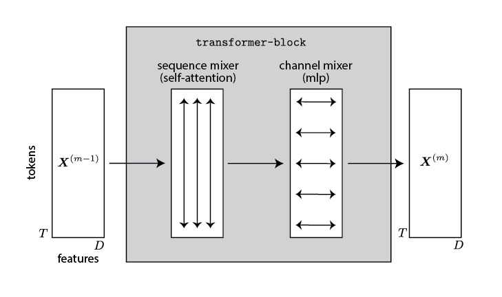
The output results from a stack of transformer blocks,

Each block consists of two stages: one that operates vertically, combining information across the sequence length; another that operates horizontally, combining information across feature dimensions.

Attention¶

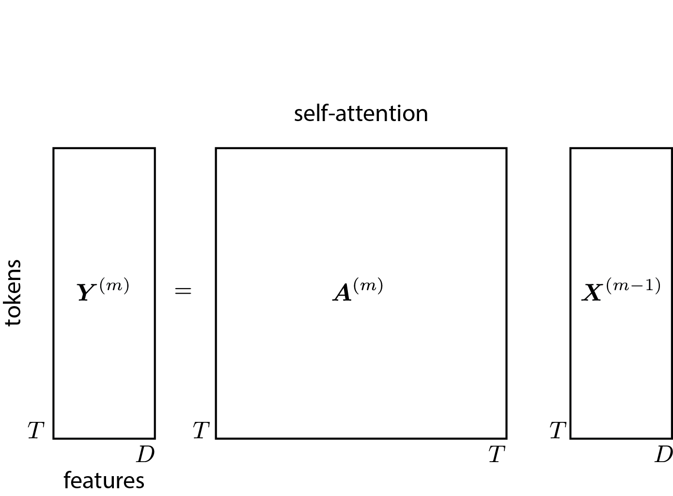
The first stage combines information across sequence length using a mechanism called attention. Mathematically, attention is a weighted average,

where $\mbA^{(\ell)} \in \reals_+^{T \times T}$ is a row-stochastic attention matrix: $\sum_{s} A_{ts}^{(\ell)} = 1$ for all $t$. Intuitively, $A_{t,s}^{(\ell)}$ indicates how much output location $t$ attends to input location $s$.

When using transformers for autoregressive sequence modeling, we constrain the attention matrix to be causal by requiring $A_{t,s}^{(\ell)} = 0$ for all $s > t$ — i.e., the matrix is lower triangular.

Self-Attention¶

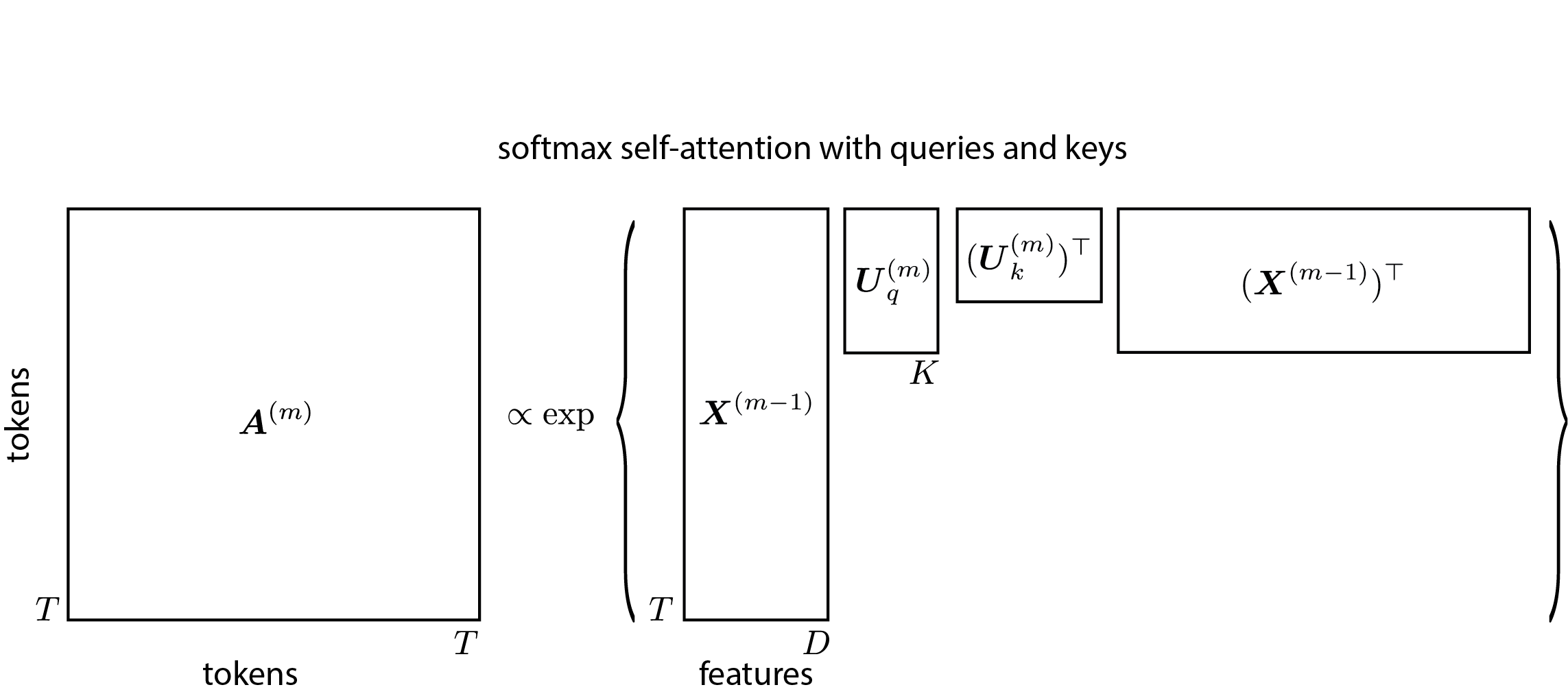
Where does the attention matrix come from? In a transformer, the attention weights are determined by the pairwise similarity of tokens in the sequence. The simplest instantiation would be

(We drop the superscript ${}^{(\ell)}$ for clarity in this section.)

In practice, different feature dimensions convey different kinds of information. Transformers use separate linear projections for the queries and keys:

where $\mbW_q \mbx_t \in \reals^{K}$ are the queries, $\mbW_k \mbx_s \in \reals^{K}$ are the keys, and the $1/\sqrt{K}$ factor prevents the dot products from growing large in magnitude Vaswani et al., 2017.

The KV Cache¶

During autoregressive generation, the model produces one token at a time. At step $t$, all keys $\mbW_k \mbx_{s}$ and values $\mbW_v \mbx_{s}$ for $s < t$ were already computed at previous steps. Rather than recomputing them, an efficient implementation stores them in a KV cache and retrieves them when generating each new token. This reduces the per-step cost from $O(t D^2)$ to $O(D^2)$, but the cache grows linearly with context length — a key memory bottleneck at inference time.

Multi-Headed Self-Attention¶

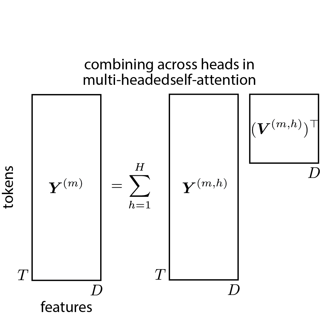
Just as a CNN uses a bank of filters in parallel, a transformer block uses $H$ attention heads in parallel. Let

where

for $h = 1, \ldots, H$. The outputs are projected and summed:

where $\mbW_o^{(\ell,h)} \in \reals^{D \times K}$ maps each head’s output back to the token dimension.

The Residual Stream¶

The residual connections in a transformer — introduced as an optimization technique in He et al. (2016) — have a deeper architectural interpretation. Writing out the full forward pass,

reveals that every component — every attention head and every MLP — adds its output directly onto a shared residual stream that begins as the token embedding and accumulates updates across all layers Elhage et al., 2021.

This perspective has several consequences:

• All components read from and write to the same space. Attention heads and MLPs interact not through layer boundaries but through their shared updates to the stream. One head can write information that a later head in a different layer reads directly.

• Each head is a low-rank read-write. With the Q/K/V/O factorization, each attention head reads from the stream via $\mbW_q$ and $\mbW_k$, computes an update, and writes it back via $\mbW_o \mbW_v$ — a rank-$K$ operation on the $D$-dimensional stream.

• Residuals are structural, not incidental. The residual stream framing is the foundation of mechanistic interpretability: by analyzing which subspaces different heads and MLPs read from and write to, researchers have identified circuits that implement specific algorithms (induction, copying, retrieval) inside trained transformers.

Token-wise Nonlinearity¶

After the multi-headed self-attention step, the transformer applies a token-wise nonlinear transformation to mix feature dimensions. This is done with a feedforward network applied identically at each position,

Mixture of Experts¶

A mixture of experts (MoE) layer replaces the single MLP at each transformer block with $E$ independent “expert” MLPs and a learned router that selects a sparse subset of them for each token Shazeer et al., 2017. Given a token $\mby_t$, the router computes a probability over experts,

and routes the token to the top-$k$ experts (typically $k = 1$ or $k = 2$):

Because only $k \ll E$ experts are active per token, the computation per token is the same as a dense model with a single MLP — but the total number of parameters scales with $E$. This decoupling of parameter count from compute allows MoE models to reach much higher capacity for the same training FLOP budget. Fedus et al. (2022) showed that even $k = 1$ (routing each token to a single expert) works well at scale; modern deployments such as Mixtral 8×7B use $E = 8$ experts with $k = 2$. The main practical challenges are load balancing (ensuring tokens are spread roughly evenly across experts, typically enforced with an auxiliary loss) and the communication overhead of routing tokens to different devices in a distributed setting.

Layer Norm¶

LayerNorm stabilizes training by z-scoring each token and applying a learned shift and scale:

where $\mbbeta, \mbgamma \in \reals^D$ are learned parameters. LayerNorm is applied before each sub-layer (Pre-LN), which yields more stable training than the original Post-LN design:

This defines one $\texttt{transformer-block}$. A transformer stacks $L$ such blocks to produce a deep sequence-to-sequence model.

Positional Encodings¶

Without explicit position information, a transformer treats its inputs as an unordered set of tokens — the architecture is permutation-equivariant (subject only to the causal mask). When the data have spatial or temporal structure, position must be injected explicitly.

Absolute Positional Encodings¶

The original transformer adds a fixed position vector to each token embedding:

where $\mbp_t \in \reals^D$ encodes the position using sinusoidal basis functions Vaswani et al., 2017. Learned absolute position embeddings are also common.

Rotary Position Embeddings (RoPE)¶

Absolute encodings bake position into the token embedding before the attention computation, which limits the model’s ability to generalize to sequence lengths unseen during training. Rotary Position Embeddings (RoPE) Su et al., 2024 instead encode position directly into the query–key dot product by rotating query and key vectors before the inner product.

Concretely, partition the $K$-dimensional query and key into $K/2$ pairs of consecutive dimensions. For pair $i$, define the $2 \times 2$ rotation matrix,

with base frequencies $\theta_i = b^{-2i/K}$ for a large base $b$ (commonly $b = 10000$). Apply these rotations elementwise to the query and key before computing attention weights:

Because $(\mbR_t \mbq_t)^\top (\mbR_s \mbk_s) = \mbq_t^\top \mbR_t^\top \mbR_s \mbk_s = \mbq_t^\top \mbR_{t-s} \mbk_s$, the dot product depends only on the relative position $t - s$. This relative-position property makes RoPE extrapolate more gracefully to longer sequences than absolute encodings. RoPE is now the dominant positional encoding in open-weight LLMs (LLaMA, Mistral, Qwen, Gemma).

Autoregressive Modeling¶

To use a transformer for autoregressive modeling, predictions are read from the final layer’s representations. To predict the next token label $z_{t+1} \in \{1,\ldots,V\}$ given past tokens $z_{1:t}$:

where $\mbW_u \in \reals^{V \times D}$ is the unembedding matrix. Like hidden states in an RNN, the final-layer representations $\mbx_t^{(L)}$ aggregate information from all tokens up to index $t$.

Training¶

Standard practice is to use the AdamW optimizer with gradient clipping, a warmup-then-cosine learning rate schedule, and dropout. Treat these as hyperparameters; the optimal settings are model- and data-dependent.

Scaling Laws¶

One of the most practically useful findings in LLM research is that validation loss follows power-law scaling in model size $N$ (number of parameters) and dataset size $D$ (number of training tokens) Kaplan et al., 2020. The loss decreases smoothly as either resource grows, with the two contributions approximately additive — meaning a bottleneck on one resource cannot be compensated by adding more of another.

An immediate consequence is that for a fixed compute budget $C \approx 6ND$ FLOPs, there is an optimal allocation between model size and training tokens. Kaplan et al. (2020) initially argued that model size should be prioritized, leading to the practice of training large models on relatively few tokens. Hoffmann et al. (2022) revisited this with more careful experiments and found that model size and training tokens should scale in roughly equal proportion: the Chinchilla result is that the compute-optimal number of training tokens is approximately $D^* \approx 20N$. Concretely, a 7B-parameter model trained compute-optimally should see around 140B tokens — much more data than earlier models of comparable size used.

This has had an outsized practical impact: post-Chinchilla models (LLaMA and its successors) train smaller models on far more data than pre-Chinchilla norms, achieving better performance at inference time for the same training compute.

Open-Weight LLMs¶

The transformer landscape is evolving too rapidly for any static summary to remain useful for long. That said, students interested in working with LLMs directly have access to a growing ecosystem of high-quality open-weight models — models whose weights are publicly released even if training details are not always fully disclosed. Current families worth being aware of include Meta’s LLaMA series Touvron et al., 2023Grattafiori et al., 2024, Mistral AI’s Mistral and Mixtral models Jiang et al., 2023Jiang et al., 2024, Google’s Gemma family Gemma Team, 2024, and Alibaba’s Qwen series. These span a range of sizes (1B–405B parameters) and are available through Hugging Face, Ollama, and similar platforms. All of them implement the core building blocks described in this chapter — Pre-LN, RoPE, GQA, and SwiGLU — with the main differences lying in scale, training data, and fine-tuning for instruction following.

Conclusion¶

Transformers achieve parallelism over a full sequence by replacing the sequential hidden-state recursion with multi-headed self-attention: each token directly attends to all previous tokens, enabling gradient information to flow in a single step rather than through $T$ chained Jacobians. Viewing the architecture through the lens of the residual stream clarifies that attention heads and MLPs all operate on a shared representational space, with each component contributing a low-rank additive update. The quadratic $O(T^2)$ cost of softmax attention is a practical bottleneck for long sequences and has motivated substantial recent work on more efficient alternatives.