Markerless Pose Tracking#
We’ve talked a lot about extracting neural signals from ephys and ophys measurements, but what comes next? One of the fundamental goals of systems neuroscience is to understand the relationship between neural activity and behavioral outputs. To that end, we need to quantify and model not only neural activity but animals’ behavior as well.
The study of natural behavior is called ethology [Tinbergen, 1963]. With advances in deep learning, the field is undergoing a computational revival [Anderson and Perona, 2014]. The once tedious process of labeling video data to track body posture and annotate behaviors has been largely automated by machine learning methods, which are well-suited to the task [Bala et al., 2020, Branson et al., 2009, Graving et al., 2019, Machado et al., 2015, Mathis et al., 2018, Pereira et al., 2022, Wu et al., 2020]. At the intersection of computational neuroscience and computational ethology is the (predictably named) emerging field of computational neuroethology [Datta et al., 2019].
This chapter develops the basic methods underlying most markerless pose tracking systems. There are a few key ideas. First, we can cast pose tracking — i.e. the task of labeling keypoints of interest in video frames, like an animals paws, snout, and tail, and tracking them over time — as a supervised learning problem. Given a few labeled frames, we can train a classifier to predict the keypoint locations in new frames. Second, such classifiers require surprisingly few training examples, particularly when they are given features from networks that have been pre-trained on similar tasks. For example, deep neural networks trained for image classification on very large datasets like ImageNet may not immediately solve pose tracking problems, but the features they’ve learned for classifying cats and dogs may still be useful for tracking paws and snouts. Using a neural network trained on one task to jump-start a model for a similar task is called transfer learning.
We’ll start with a simple logistic regression model for pose tracking and show how it can be implemented with a convolutional neural network (CNN). Then we’ll show how the same ideas can be generalized to pre-trained CNNs for image classification, like very deep residual networks [He et al., 2016].
Supervised learning#
In supervised learning problems, our data consists of a set of tuples \(\{(\mathbf{x}_n, y_n)\}_{n=1}^N\) where \(\mathbf{x}_n\) are the inputs and \(y_n\) are the outputs. Contrast this with the spike sorting and calcium deconvolution problems, which we framed as unsupervised matrix factorization problems.
A simple way to frame the pose tracking problem as a supervised learning problem is to chop each image frame into patches and then assign each patch a binary label to indicate whether or not the patch contains a specific key point (e.g. “left paw”). Then we can train a binary classifier to predict the labels given the image patches. Of course, we usually want to track multiple key points at once, and we could simply train separate classifiers for each one. Ideally, the trained classifiers will generalize to new image patches from new video frames, giving us predictions about which patches contain which keypoints. Then, in post-processing, we can determine the most likely configuration of key points in future frames, using the classifiers’ predictions.
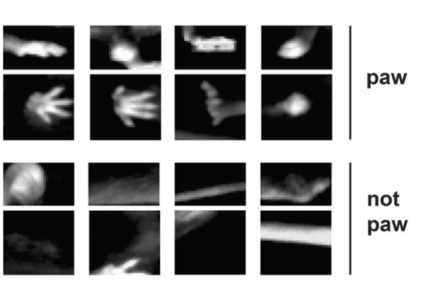
Fig. 9 A simple way to do pose tracking is to carve each video frame into small patches and label them as positive or negative examples of a key point. Then train a classifier to predict the label for new patches. This figure was adapted from fig. 1B of Machado et al. [2015]#
Logistic regression#
Let \(\mathbf{x}_n \in \mathbb{R}^P\) be the \(n\)-th image patch, flattened into a vector of \(P\) pixels. Let \(y_n \in \{0,1\}\) be a binary label specifying whether the key point of interest is present in that frame.
In logistic regression, we model the conditional distribution of the label given the image as,
where \(\mathbf{w} \in \mathbb{R}^P\) are the weights for each pixel, and \(\sigma: \mathbb{R} \mapsto (0, 1)\) is the logistic function
The Bernoulli distribution
The Bernoulli distribution is a distribution over binary variables \(y \in \{0,1\}\) with probability \(p \in [0,1]\). Its pmf can be written as,
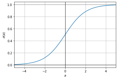
The logistic (sigmoid) function
The logistic (aka sigmoid) function is a map from the reals to the interval \((0,1)\). It is defined as,
It asymptotes at \(\lim_{a \to -\infty} \sigma(a) = 0\) and \(\lim_{a \to \infty} \sigma(a) = 1\). It is plotted below.
Interestingly, the logistic function is symmetric in that,
Its derivative is,
The derivative is positive (i.e., the logistic function is monotonically increasing) and attains its maximum at \(\sigma'(0) = \tfrac{1}{4}\).
Show code cell source
import torch
import matplotlib.pyplot as plt

aa = torch.linspace(-5, 5, 100)
plt.plot(aa, torch.sigmoid(aa))
plt.axhline(0, color='k', lw=1)
plt.axhline(1, color='k', ls=':', lw=1)
plt.axvline(0, color='k', lw=1)
plt.grid("True")
plt.xlim(-5, 5)
plt.xlabel(r"$a$")
_ = plt.ylabel(r"$\sigma(a)$")
Optimization#
Our goal is to estimate the weights \(\mathbf{w}_{\mathsf{MLE}}\) that maximize the log likelihood of the training data, or equivalently minimize the negative log likelihood. Unlike most of the problems we’ve encountered thus far, we won’t have a closed form solution for the weights, even if we try to do coordinate ascent. Instead we’ll have to turn to more general optimization strategies like gradient descent and Newton’s method. This is a good opportunity to introduce a few of these tools and some of the key concepts.
Setup#
Let \(\mathbf{X} \in \mathbb{R}^{N \times P}\) denote the matrix of inputs (with rows \(\mathbf{x}_n^\top\)) and \(\mathbf{y} = (y_1, \ldots, y_N) \in \{0,1\}^N\) denote the vector of output labels. The negative log likelihood is,
The gradient with respect to the weights#
The gradient with respect to \(\mathbf{w}\) is,
Unfortunately, this is a nonlinear function of \(\mathbf{w}\) (due to the logistic function), and when we set to zero and try to solve for the weights, we find there is no closed-form solution.
The negative log likelihood is convex#
While there may not be a closed-form solution, the problem is not necessarily all that hard to solve. It turns out the negative log likelihood is a convex function of the weights — i.e., it looks like an upward facing bowl — so we can solve it with off-the-shelf optimization tools.
To show that the objective function is convex, it suffices to show that it is twice-differentiable and its Hessian (the matrix of second-order partial derivatives) is positive semi-definite (has eigenvalues \(\geq 0\)).
The Hessian of the negative log likelihood is,
where \(\sigma'(\mathbf{w}^\top \mathbf{x}_n)\) is the derivative of the logistic function (see above) evaluated at \(\mathbf{w}^\top \mathbf{x}_n\).
Since this a sum of outer products (\(\mathbf{x}_n \mathbf{x}_n^\top\)) with positive coefficients (\(\sigma(\mathbf{w}^\top \mathbf{x}_n)\)), the Hessian is positive semi-definite.
Matrix derivatives
It takes some practice to become familiar with the rules of matrix calculus. I recommend the first chapters of The Matrix Cookbook [Petersen et al., 2008] for an introduction.
Gradient descent#
Since the the negative log likelihood is convex (equivalently, the log likelihood is concave), we have a host of tools at our disposal for maximum likelihood estimation. We don’t need CVXPy to solve this problem (like we did for the previous chapter). Here, we can simply perform gradient descent.
Let \(\mathbf{w}_0\) denote our initial setting of the weights. Gradient descent is an iterative algorithm that produces a sequence of weights \(\mathbf{w}_0, \mathbf{w}_1, \ldots\) that (under certain conditions) converges to a local optimum of the objective. Since the objective is convex, all local optima are global optima. The idea is straightforward, on each iteration we update the weights by taking a step in the direction of the gradient,
where \(\alpha_i \in \mathbb{R}_+\) is the learning rate (aka step size) on iteration \(i\), and \(\nabla \mathcal{L}(\mathbf{w}_i)\) is the gradient of the objective evaluated at the current weights \(\mathbf{w}_i\).
Convergence of gradient descent
When \(\mathcal{L}\) is convex and \(\nabla \mathcal{L}\) is Lipschitz continuous, and when the learning rates satisfy certain conditions (e.g., they are set by a backtracking line search), then gradient descent will converge to a local optimum. When the objective is convex, all local optima are global optima, so then gradient descent is guaranteed to find a global solution.
Newton’s method#
Gradient descent uses first-order information (i.e., the gradient of the objective at the current weights) to determine the descent direction. We can obtain faster convergence rates using second-order information (i.e., the Hessian of the objective).
The idea is to minimize a quadratic approximation of the objective given by a Taylor approximation around the current weights,
The minimum of this quadratic approximation has a closed form solution,
Here, the descent direction is given by the inverse-Hessian times the gradient, \(\nabla^2 \mathcal{L}(\mathbf{w}_i)^{-1} \nabla \mathcal{L}(\mathbf{w}_i)\).
Warning
Note that Newton’s method assumes that the Hessian is invertible, which is almost surely the case for logistic regression with many data points. We can ensure invertibility by adding a multivariate normal prior on the weights, as we will introduce below.
Newton’s method can be unstable in practice. A simple fix is to use the same descent direction, but that to vary the step size \(\alpha_i\),
For example, the step-size can be set to \(\alpha_i < 1\) to implement damped Newton’s method, or it can be determined by a backtracking line search.
Iteratively reweighted least squares (IRLS)#
The weight updates simplify nicely when we substitute in the form of the gradient and Hessian for logistic regression. Note that they can be written in matrix form as,
where
is a diagonal scaling (aka weighting) matrix. Note that the scale factors are all positive since \(\sigma'(a) > 0\).
Substituting these forms in and rearranging yield,
where
In other words, the standard Newton method update can be viewed as the solution to a weighted least squares problem with weights \(\mathbf{S}\) and targets \(\tilde{\mathbf{y}}\) that depend on the current weights \(\mathbf{w}_i\). Viewed this way, we see that Newton’s method for logistic regression is equivalent to an algorithm called iteratively reweighted least squares (IRLS).
Computational complexity#
Exercise
Show that the computational complexity of gradient descent is \(\mathcal{O}(NP)\) whereas the complexity of Newton’s method is \(\mathcal{O}(NP^2 + P^3)\).
Scaling up#
Though it converges faster, Newton’s method quickly becomes intractable for large \(N\) and \(P\). For large \(N\), even gradient descent becomes costly. There are a few ways to speed up computation:
Quasi-Newton methods like BFGS replace the exact Hessian with an approximation and side-step the explicit matrix inversion.
Stochastic gradient descent (SGD) uses subsets of data (a.k.a. minibatches) to approximate the gradient. Under fairly general conditions, it converges to a local optimum.
Momentum is often used in conjunction with SGD to keep the descent direction from changing too rapidly. This can address some of the limitations of regular gradient descent as well, e.g., where the updates overshoot in poorly conditioned problems. Related methods like Nesterov’s accelerated gradient (see Sutskever et al. [2013]) can achieve second-order convergence rates using first-order information (under certain conditions).
Still, SGD (with momentum) requires setting a learning rate. Modern machine learning packages like
torch.optimimplement a number of optimizers that automatically tune the learning rates, like AdaGrad [Duchi et al., 2011], RMSProp [Hinton et al., 2014], and Adam [Kingma and Ba, 2014].
Pose tracking with convolutional neural networks (CNNs)#
Remember we started by treating each data point as patch \(\mathbf{x}_n\) and a binary label \(y_n\) specifying whether a specific key point (e.g. “left paw”) is present. Of course, in practice we want to classify all the patches in an image in parallel, and we want to predict more than one type of key point.
Let \(\mathbf{X}_n \in \mathbb{R}^{P_H \times P_W}\) denote the \(n\)-th image and \(\mathbf{Y}_{n,k} \in \{0,1\}^{P_H \times P_W}\) denote the binary mask of where in the \(k\)-th key point is in the \(n\)-th image. Both are \(P_H\) pixels in height and \(P_W\) pixels wide. Assume the patches are \(P_h \times P_w\) in size, with \(P_h < P_H\) and \(P_w < P_W\). Finally, ket \(\mathbf{W}_k \in \mathbb{R}^{P_h \times P_w}\) denote the weights for the \(k\)-th key point.
We can think of each image as having \(P_H \cdot P_W\) patches and corresponding labels, one centered on each pixel. In our simple logistic regression model, each patch’s label is modeled as a conditionally independent Bernoulli random variable,
where \(a_{n,k,i,j} \in \mathbb{R}\) is the activation for that specific image, key point, and pixel. The activations are given by a 2D cross-correlation,
In fact, the activations for an entire batch of \(N\) images and \(K\) key points (i.e., output channels) can be computed in a single call to F.conv2d, with the appropriate padding. In lab, we’ll make use of the torch.nn.Conv2d class, which encapsulates the weights of a 2D convolution layer and makes it easy to train such models.
Convolutional neural networks#
Framed this way, we can view the logistic regression model as a one-layer convolutional neural network (CNN). This view also suggests an obvious direction for improvement. The activations of the logistic regression model are linear functions of the pixels. In practice, a good key point detector may need nonlinear features of the images. Moreover, the features necessary to predict one keypoint (e.g., the left paw) may be similar to those needed for another (e.g., the right).
Convolutional neural networks allow both nonlinear feature learning and feature sharing between outputs. The idea is straightforward: stack multiple convolutional layers on top of each other, feeding the output of one as the input to the next.
Residual networks (ResNets) enable very deep CNNs to be stably trained by adding skip connections whereby the input is fed straight to the output of a layer, thereby allowing the convolution to capture the difference (i.e., residual) between the input and output.
These notes will not comprehensively cover CNNs and ResNets. Instead, please consult the many great online resources, like Goodfellow et al. [2016] and the PyTorch tutorials.
Working with minimal labeled data.#
While deep neural networks like CNNs and ResNets have the capacity to learn nonlinear mappings from images to key point predictions, they also have many free parameters to train.
For modern machine learning tasks and benchmarks, these models are trained on millions of labeled images, like the ImageNet dataset for image classification.
Unfortunately, we don’t (yet) have comparable datasets of labeled images of animals in the lab (however, see Marshall et al. [2021]) Moreover, environments change from one lab to the next, making it challenging to collect one dataset that covers all the bases.
Ideally, we would like to train a pose tracking model for a specific lab environment using minimal labeled data.
Modern methods for markerless animal pose tracking take two approaches:
Use a lightweight architecture with fewer free parameters, like the modular UNet in SLEAP [Pereira et al., 2022]
Use transfer learning to adapt the weights of a pre-trained network to the problem of animal pose tracking [Mathis et al., 2018].
Transfer learning#
Transfer learning is when you take a model trained for one task (e.g. a ResNet trained for image classification with ImageNet) and adapt it to another task (e.g. classifying key points in behavioral video). If the tasks are similar enough, then it may require new minimal training data to adapt the pre-trained network.
For example, DeepLabCut [Mathis et al., 2018] originally converted a ResNet-50 (a very deep CNN) trained on ImageNet by rerouting the output of a middle layer to make predictions about key point locations in animal videos. We can think of the activations at the middle layer as a highly nonlinear feature bank that represents the original image in a form that may be more amenable to key point prediction with simple models.
Finally, using a small number (100s) of hand-labeled video frames, DLC can train the mapping from intermediate features to key point predictions. It can also fine-tune the weights of the ResNet to obtain very good accuracy in key point prediction.
There are, of course, many details and design questions to answer. Which layer of the ResNet do you reroute? How complex is the mapping from features to predictions? How big should you make the prediction targets? We will work through these concerns in Lab 3.
Structured prediction#
The output of these CNNs is a map of key point probabilities for each image, key point, and pixel. However, the key points are obviously not independent — knowing where the left elbow is tells you a lot about where the left shoulder is likely to be found. Ideally, we would like to make a unified prediction about the collection of key point locations.
One way to tackle this problem is with structured prediction [Felzenszwalb and Huttenlocher, 2005, Insafutdinov et al., 2016]. Let \(\ell_{n,k} \in [0,P_h] \times [0,P_w]\) be a random variable denoting the location of key point \(k\) in image \(n\) (in pixel coordinates). We can represent a joint distribution over the collection of key points \(\boldsymbol{\ell}_n = (\ell_{n,1}, \ldots, \ell_{n,K})\) as a factor graph,
where \(f_k\) are called unary potentials and \(g_{ij}\) are called pairwise potentials. The unary potentials are functions that specify how likely key point \(k\) is to be found at a location \(\ell_{n,k}\) given the observed image \(\mathbf{x}_n\); the pairwise potentials specify how likely the joint configuration of \((\ell_{n,i}, \ell_{n,j})\) is. For example, the pairwise potentials could rule out configurations in which the left elbow is meters away from the left shoulder.
Note that this joint distribution is unnomrmalized. That isn’t a problem for maximuim a posteriori (MAP) estimation of the key point locations, but it does make learning the parameters of the potential functions a bit harder. We’ll come back to this later in the course.
3D Triangulation#
Finally, we have so far focused on finding key points in 2D images, but there is growing interest in tracking 3D pose from multiple camera views.
One way to solve this problem is by training a CNN that synthesizes multiple 2D views into a 3D representation [Dunn et al., 2021]. Another is to use triangulation to infer a 3D key point location from multiple 2D views [Karashchuk et al., 2021, Nath et al., 2019, Zhang et al., 2021].
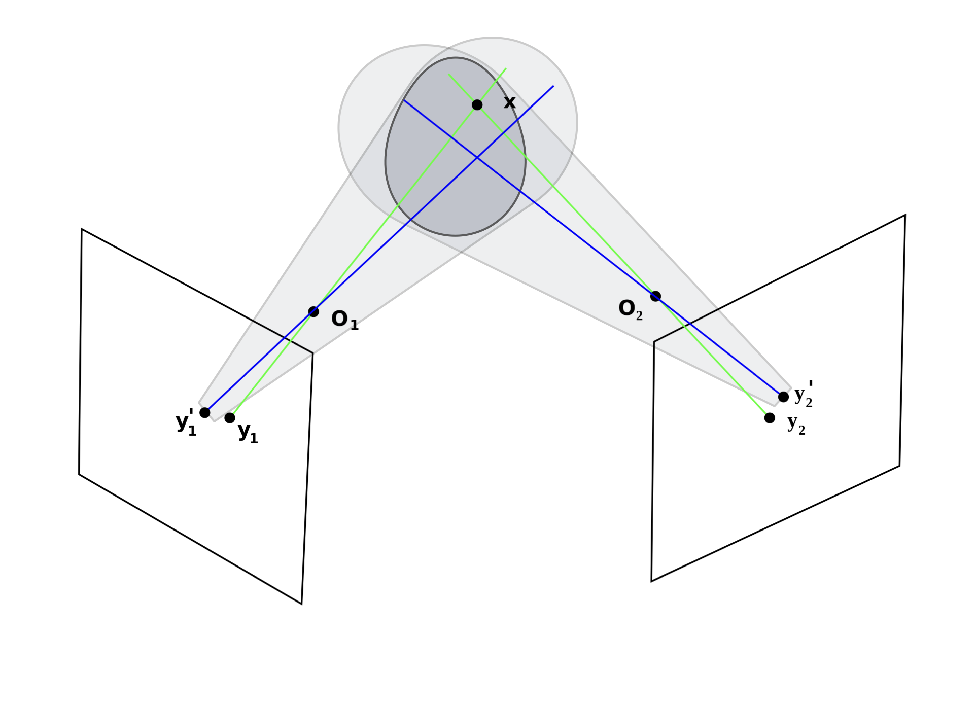
Fig. 10 Projective geometry makes far away objects appear smaller. Image modified from Wikipedia.#
GIMBAL [Zhang et al., 2021] combines structured prediction and triangulation to infer 3D pose from multiple 2D key point estimates. Changing notation slightly, let \(\mathbf{y}_{c,k} \in \mathbb{R}^2\) denote the estimated location of key point \(k\) in the coordinates of camera \(c\), and let \(\mathbf{x}_k \in \mathbb{R}^3\) denote the 3D location in “world coordinates.” Projective geometry tells how to map 3D locations to 2D images,
where
are the 3D coordinates after affine transformation (parameterized by \(\mathbf{A}_c\) and \(\mathbf{b}_c\)) into the frame of camera \(c\). Note that the transformation is nonlinear due to the scaling by \(w^{-1}\).
GIMBAL combines this nonlinear camera model with a structured prior distribution on 3D key point locations \(\mathbf{x} = (\mathbf{x}_1, \ldots, \mathbf{x}_K)\) obtained from a hierarchical von Mises-Fisher-Gaussian distribution.
Conclusion#
This chapter introduced the basics of modern animal pose tracking methods using supervised learning, deep convolutional neural networks, transfer learning, and structured prediction. Many of these techniques will reappear later in the course as we talk about encoding and decoding neural spike trains. In lab, you will practice implementing these techniques and building a simple pose tracker.
Further reading#
As always, there is much more to say on each of the topics covered in this chapter. There is growing work on semi-supervised pose tracking to leverage the wealth of unlabeled image frames [Whiteway et al., 2021, Wu et al., 2020]. There is still work to be done on multi-animal pose tracking [Lauer et al., 2022, Pereira et al., 2022], and recent machine learning challenges like MABe have sought to make progress on these problems. Finally, experimentalists are starting to use these kinds of techniques for real-time pose tracking to guide closed-loop optogenetic stimulation of neural circuits [Markowitz et al., 2023]. While there is still room for methodological improvement, these methods have already transformed the landscape of systems neuroscience.